MSA-based pLMs encode evolutionary distance but don’t reliably exploit it –

NoteAI usage disclosure

We used Claude (Sonnet 4.5) to help write, clean up, and comment our code; we also used it to review our code and selectively incorporated its feedback. Additionally, we used Gemini (3.0 Pro) to suggest wording ideas and then chose which small phrases or sentence structure ideas to use, write text that we edited, rearrange starting text to fit the structure of one of our pub templates, expand on summary text that we provided and then edited the text it produced, and help copy-edit draft text to match Arcadia’s style.

Purpose

Auditing the evolutionary information encoded by MSA Pairformer is a critical step in understanding the behavior of protein language models (pLMs) that leverage external context in the form of MSAs. In this study, we bridge MSA Pairformer with classical phylogenetics to quantify how the model’s internal sequence weighting maps onto inferred phylogenetic trees. We show that while MSA Pairformer effectively encodes evolutionary relatedness, and does so in specific layers, this signal is a subtle optimization rather than a load-bearing pillar for contact prediction accuracy. This work is intended for biologists and model developers seeking to interpret how evolutionary history is represented within pLMs. It provides a framework for evaluating the “phylogenetic operating range” of MSA-based models and highlights the need for future architectures to selectively gauge input signal reliability.

Introduction

The current trajectory of protein language modeling is dominated by a drive toward massive parameter scaling. Models such as ESM2 (Lin et al., 2023) have achieved strong performance by internalizing the evolutionary statistics of protein families within billions of learned weights. However, as sequence databases expand at a rate that outpaces feasible computational growth, this “memorization” through scaling faces a significant sustainability challenge (Akiyama et al., 2025).

MSA-based architectures, such as MSA Transformer (Rao et al., 2021) and the more recent MSA Pairformer (Akiyama et al., 2025), represent a pivot toward models that utilize external evolutionary context as input. By extracting information directly from multiple sequence alignments (MSAs) passed as input to the model at runtime, these models shift the burden of knowledge from fixed parameters to the specific sequences provided in the MSA, allowing for high performance with significantly fewer model parameters. Yet, this shift introduces a new architectural hurdle: resolving specific structural signals within a divergent alignment without diluting them through phylogenetic averaging¹.

¹ A limitation in MSA-based models whereby sequences are treated as independent of one another, disregarding their evolutionary relatedness to one another. By treating divergent lineages as if they share an identical structure, this process dilutes subfamily-specific signals, like distinct binding interfaces, which can obscure unique evolutionary constraints of the query sequence.

² In MSA Pairformer, each MSA has one sequence-of-interest, denoted as the “query.”

MSA Pairformer addresses this via a query-biased attention mechanism, positing that performance is maximized when the model can selectively weight sequences based on their specific evolutionary relevance to the query². However, evolutionary relevance is vague and lacks a precise metric.

To address this ambiguity, we investigate if evolutionary relatedness (measured as patristic distance³ on a phylogenetic tree) serves as a quantifiable correlate of these sequence weights. While the input MSA implicitly encodes phylogenetic history, it remains to be seen if the model actively leverages this biological signal, or if it instead relies on alternative statistical heuristics to build its representations. Distinguishing between these possibilities is critical for determining if the model’s representations are grounded in evolutionary logic as purported, and if this grounding is a causal driver of downstream performance. While the original paper showed that attention weights could separate subfamilies, this was not a fully-fledged characterization of how sequence weights map onto phylogenetic structure, and was demonstrated for just one protein family. This leaves open the question of how accurately the model’s attention mechanism recapitulates evolutionary relatedness and how broadly these patterns hold across diverse protein families.

³ Patristic distance is the distance between two tips/leaves of a phylogenetic tree, calculated as the sum of branch lengths connecting them. Mathematically, \(d_{ij} = \sum_{b \in P_{ij}} l(b)\), where \(P_{ij}\) is the shortest path through the phylogeny connecting taxa \(i\) and \(j\), and \(l(b)\) is the length of branch \(b\).

In this work, we explore these questions directly. We begin by reanalyzing the response regulator (RR) protein family case study presented by Akiyama et al. (2025), and then expand our investigation to thousands of MSAs of diverse protein families spanning the tree of life. Our goal is to scope out the anatomy of the model’s learning of evolutionary distance and how it relates to downstream performance.

Revisiting the response regulator study

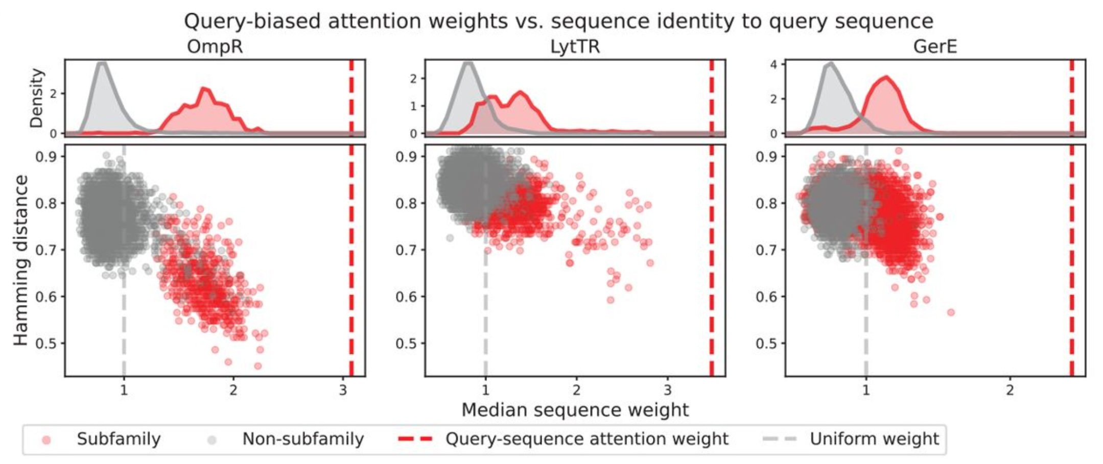
The response regulator (RR) family was the original paper’s showcase for demonstrating the power of query-biased attention. By constructing a mixed MSA of GerE, LytTR, and OmpR subfamilies, the authors showed MSA Pairformer could successfully identify key structural contacts unique to each subfamily.

They illustrated one potential mechanism behind this success by plotting model sequence weights against Hamming distance⁴, revealing that members of the query’s subfamily were consistently upweighted, leading to an inverse correlation between Hamming distance (a proxy for evolutionary distance) and sequence weight, as shown below.

⁴ Hamming distance is the number of positions at which two sequences of equal length differ.

Figure 4B from Akiyama et al. (2025). Original caption: “Median sequence weight across the layers of the model versus Hamming distance to the query sequence. Top panels show distribution of sequence attention weights for subfamily members (red) and non-subfamily sequences (grey). The grey dotted line indicates weights used for uniform sequence attention and the red dotted line indicates weight assigned to the query sequence.”

We can build on this analysis by replacing the proxy of Hamming distance with a formal phylogenetic tree inferred from the input MSA, which would allow us to ask a more nuanced question: Do the model’s sequence weights recapitulate the continuous evolutionary distances among individual sequences, or do they more closely resemble a binary distinction between “in-group” and “out-group”?

To ground our phylogenetic analysis in the paper’s original findings, we start by replicating the dataset. Following the protocol laid out by Akiyama et al. (2025), we begin by downloading the full PFAM alignments for the GerE, LytTR, and OmpR subfamilies, combining them, and then sampling a final set of 4096 sequences to match the dataset used in the study.

NoteReproducing the response regulator MSAs

Akiyama et al. (2025) qualitatively describe how to reproduce the response regulator MSAs, however these details are insufficient for exact replication. The code below is our attempted reproduction, and we find these MSAs yield similar, yet not identical, sequence weight statistics.

from collections import Counter
from pathlib import Path

import pandas as pd
from MSA_Pairformer.dataset import MSA

from analysis.pfam import download_and_process_response_regulator_msa

response_regulator_dir = Path("./data/response_regulators")
response_regulator_dir.mkdir(parents=True, exist_ok=True)

rr_msas: dict[str, MSA] = {}
rr_queries = {"1NXS": "OmpR", "4CBV": "LytTR", "4E7P": "GerE"}
for query in rr_queries:
    msa_path = response_regulator_dir / f"PF00072.final_{query}.a3m"

    if not msa_path.exists():
        download_and_process_response_regulator_msa(
            output_dir=response_regulator_dir,
            subset_size=4096,
        )

    rr_msas[query] = MSA(msa_file_path=msa_path, diverse_select_method="none")

example_msa = rr_msas[query]
membership_path = response_regulator_dir / "membership.txt"
target_to_subfamily = (
    pd.read_csv(membership_path, sep="\t").set_index("record_id")["subfamily"].to_dict()
)

print(f"MSA has {len(example_msa.ids_l)} sequences:")

subfamily_member_count = Counter()
for sequence in example_msa.ids_l:
    subfamily_member_count[target_to_subfamily[sequence]] += 1

for subfamily, count in subfamily_member_count.items():
    print(f"  - {subfamily} sequences: {count}")

MSA has 4096 sequences:
  - GerE sequences: 2545
  - LytTR sequences: 1087
  - OmpR sequences: 464

To infer a tree for this MSA, we use FastTree, a rapid method for approximating maximum-likelihood phylogenies suitable for trees of this size (Price et al., 2009).

NoteAccuracy concerns using FastTree

FastTree’s heuristic-based approach to maximum-likelihood inference can sacrifice accuracy compared to more exhaustive methods. We address these concerns in detail in the section, “Is FastTree accurate enough?”, where we benchmark our results against IQ-TREE to quantify the impact of tree inference quality on our findings.

from analysis.tree import read_newick, run_fasttree

fasttree_path = response_regulator_dir / "PF00072.final.fasttree.newick"
fasttree_log_path = response_regulator_dir / "PF00072.final.fasttree.log"
msa_for_tree = response_regulator_dir / "PF00072.final.fasta"
if not fasttree_path.exists():
    run_fasttree(msa_for_tree, fasttree_path, log_file=fasttree_log_path)

rr_tree = read_newick(fasttree_path)

Note

For this MSA, FastTree ends up using the Jones-Taylor-Thornton (JTT) evolutionary model with CAT approximation (20 rate categories). If you’re following along at home, you can check out the full logs at data/response_regulators/PF00072.final.fasttree.log.

Visualizing this tree provides our first direct look at the evolutionary structure of the data.

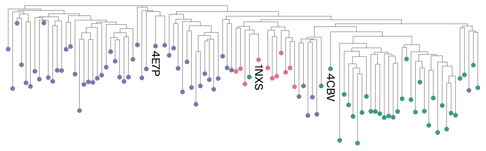
import arcadia_pycolor as apc

from analysis.plotting import tree_style_with_categorical_annotation
from analysis.tree import read_newick, subset_tree

query_colors = {
    "4E7P": apc.aster,
    "1NXS": apc.candy,
    "4CBV": apc.seaweed,
}
subfamily_colors = {rr_queries[k]: v for k, v in query_colors.items()}

tree_style = tree_style_with_categorical_annotation(
    categories=target_to_subfamily,
    highlight=list(rr_queries),
    color_map=subfamily_colors,
)
visualized_tree = subset_tree(tree=rr_tree, n=100, force_include=list(rr_queries), seed=42)
visualized_tree.render("%%inline", tree_style=tree_style, dpi=300)

Figure 1: A randomly selected subset of the response regulator family illustrating the tree structure. The RCSB structure ID is labelled for the query sequence of each subfamily. Leaves are colored according to subfamily (⬤ GerE, ⬤ OmpR, ⬤ LytTR).

We expect to see largely monophyletic clades corresponding to the three subfamilies, which is more or less what we observe in Figure 1. Discrepancies from this expectation highlight the importance of clade grouping based on explicit tree inference, rather than relying on PFAM domains.

Using the phylogeny as our objective target variable, we assess whether the model’s query-biased sequence weights successfully capture evolutionary relatedness. To do this, we’ll run an MSA Pairformer inference three separate times. Each run will use a different subfamily representative as the query, yielding three distinct, query-biased sets of sequence weights.

NoteRunning MSA Pairformer…

In order to reproduce this step of the workflow, you’ll need a GPU with at least 40GB of GPU VRAM. We don’t assume you have that hardware handy, so we’ve stored pre-computed inference results (data/response_regulators/inference_results.pt), and by default, the code below will load these inference results rather than re-computing. If you have the necessary hardware and want to re-compute the inference, delete this file prior to running the cell below, and the file will be regenerated.

from typing import Any

import torch

from analysis.pairformer import run_inference

inference_results_path = response_regulator_dir / "inference_results.pt"
if inference_results_path.exists():
    rr_inference_results = torch.load(inference_results_path, weights_only=True)
else:
    rr_inference_results: dict[str, dict[str, Any]] = {}
    for query in rr_queries:
        rr_inference_results[query] = run_inference(
            rr_msas[query], return_seq_weights=True, query_only=True
        )

    torch.save(rr_inference_results, inference_results_path)

We now have our two key components: a phylogenetic tree for the RR family (our objective target variable) and the model’s sequence weights relative to each of the three subfamily queries. Before diving into a formal statistical analysis, let’s build an intuition for how the model’s attention relates to tree structure by visualizing weights directly onto the tree.

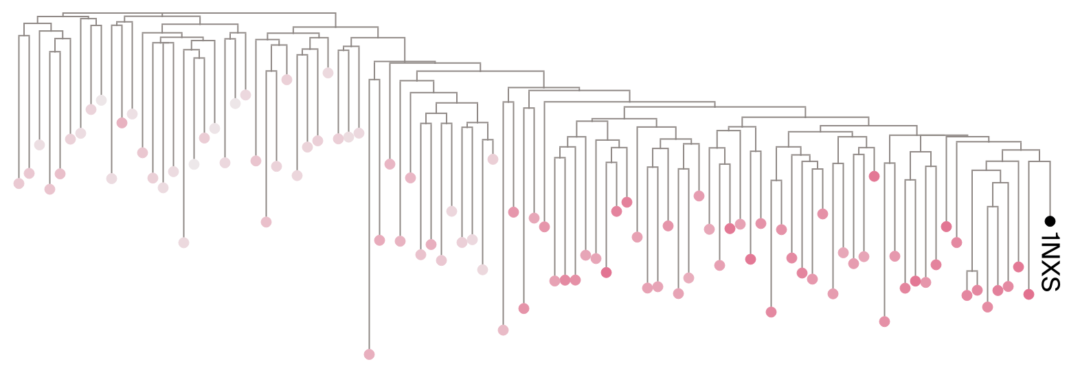
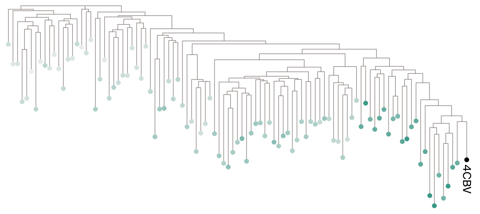
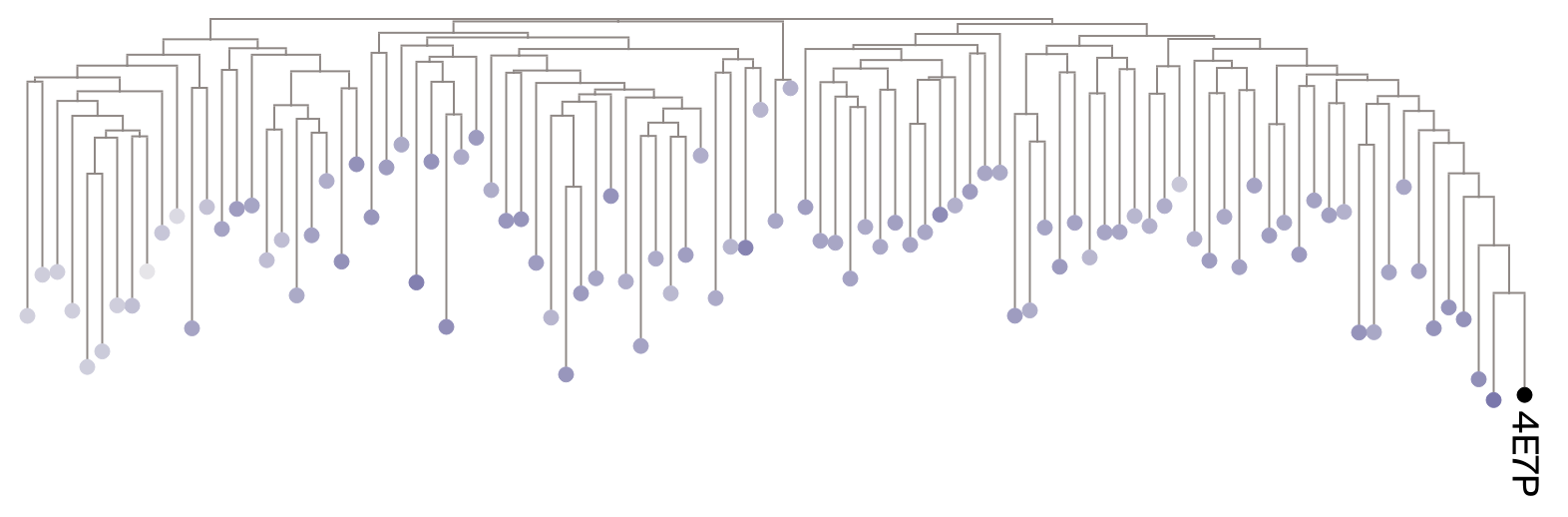
For each of the three queries, let’s center our view on a small subset of the full MSA (for ease of visualization) and color at each leaf the median (across layers) sequence weight it received from the model. If the model is capturing evolutionary relatedness, we’d expect a gradient of sequence weight that follows the tree’s branches away from the query.

from IPython.display import display

from analysis.data import get_sequence_weight_data
from analysis.plotting import tree_style_with_scalar_annotation
from analysis.tree import (
    sort_tree_by_reference,
    subset_tree_around_reference,
)

rr_data_dict = dict(
    query=[],
    target=[],
    median_weight=[],
)

for query in rr_queries:
    msa = rr_msas[query]
    targets = msa.ids_l

    weights = get_sequence_weight_data(rr_inference_results[query])

    # For each layer, sequence weights sum to 1. Scaling by number of
    # sequences yields a scale where 1 implies uniform weighting.
    weights *= weights.size(0)

    median_weights = torch.median(weights, dim=1).values

    rr_data_dict["query"].extend([query] * len(targets))
    rr_data_dict["target"].extend(targets)
    rr_data_dict["median_weight"].extend(median_weights.tolist())

response_regulator_df = pd.DataFrame(rr_data_dict)

tree_images = []
queries_list = response_regulator_df["query"].unique()
for query in queries_list:
    color = query_colors[query]
    specific_layer = "median_weight"
    specific_layer_weights = (
        response_regulator_df.loc[
            (response_regulator_df["query"] == query)
            & (response_regulator_df["query"] != response_regulator_df["target"]),
            [specific_layer, "target"],
        ]
        .set_index("target")[specific_layer]
        .to_dict()
    )

    gradient = apc.Gradient.from_dict(
        "gradient",
        {"1": "#EEEEEE", "2": "#EEEEEE", "3": color, "4": color},
        values=[0.0, 0.0, 0.75, 1.0],
    )
    tree_style = tree_style_with_scalar_annotation(
        specific_layer_weights, gradient, highlight=[query]
    )
    visualized_tree = sort_tree_by_reference(
        subset_tree_around_reference(tree=rr_tree, n=100, reference=query, bias_power=0.8, seed=42),
        query,
    )
    tree_images.append(visualized_tree.render("%%inline", tree_style=tree_style, dpi=300))

display(*tree_images)

(a) Median sequence weights with respect to 1NXS (OmpR).

(b) Median sequence weights with respect to 4CBV (LytTR).

(c) Median sequence weights with respect to 4E7P (GerE).

Figure 2: Unrooted trees for each query, where each leaf is colored according to the median sequence weight it received from the model. Darker nodes signify sequences receiving high levels of attention (upweighting), while lighter nodes signify sequences receiving low levels of attention (downweighting). Each tree is subset to 100 sequences sampled from the full tree (includes all subfamilies). To see whether we observe a gradient, sequences were sampled with a probability inversely proportional to their phylogenetic rank distance from the query, raised to a power of 0.8, which combine to give slight preference for selecting sequences phylogenetically similar to the query while still sampling across the entire phylogeny.

Encouragingly, Figure 2 provides an intuitive picture: weights with respect to 1NXS and 4CBV visually correlate with distance from the query, suggesting the model’s attention mechanism prioritizes evolutionary relatedness. However, the picture is less clear for 4E7P, which invites a quantitative test.

To formalize this observation, let’s extract the patristic distance between the queries and all the other sequences in the MSA, then compare this to the model’s median sequence weights. As in Akiyama et al. (2025), we’ll normalize weights by the number of sequences, so a value of 1 represents the uniform weighting baseline and a value greater than 1 indicates upweighting. And on the suspicion that this median value might smooth over layer-specific complexity, let’s also store the individual weights from each layer to leave room for a more granular, layer-by-layer analysis.

from scipy.stats import linregress

from analysis.data import get_sequence_weight_data
from analysis.tree import get_patristic_distance

rr_data_dict = dict(
    query=[],
    target_subfamily=[],
    target=[],
    patristic_distance=[],
    median_weight=[],
)

num_layers = 22
for layer_idx in range(num_layers):
    rr_data_dict[f"layer_{layer_idx}_weight"] = []

for query in rr_queries:
    msa = rr_msas[query]
    targets = msa.ids_l

    patristic_distances = get_patristic_distance(rr_tree, query)
    patristic_distances = patristic_distances[targets]

    weights = get_sequence_weight_data(rr_inference_results[query])

    # For each layer, sequence weights sum to 1. Scaling by number of
    # sequences yields a scale where 1 implies uniform weighting.
    weights *= weights.size(0)

    median_weights = torch.median(weights, dim=1).values

    for layer_idx in range(num_layers):
        rr_data_dict[f"layer_{layer_idx}_weight"].extend(weights[:, layer_idx].tolist())

    rr_data_dict["query"].extend([query] * len(targets))
    rr_data_dict["target_subfamily"].extend([target_to_subfamily[target] for target in targets])
    rr_data_dict["target"].extend(targets)
    rr_data_dict["median_weight"].extend(median_weights.tolist())
    rr_data_dict["patristic_distance"].extend(patristic_distances.tolist())

response_regulator_df = pd.DataFrame(rr_data_dict)
response_regulator_df = response_regulator_df.query("query != target").reset_index(drop=True)
response_regulator_df

We’ll analyze the relationship between sequence weights and patristic distance with a simple linear regression. We’ll frame the problem to directly assess the explanatory power of the model’s sequence weights: how well do they explain the patristic distance to the query?

For each query \(q\) and each target sequence \(i\) in the MSA, let’s define our model as:

\[ d_{i} = \beta_1^{(l)} w_{i}^{(l)} + \beta_0^{(l)} \tag{1}\]

where \(d_{i}\) is the patristic distance from the query \(q\) to the target sequence \(i\), \(w_{i}^{(l)}\) is the normalized sequence weight assigned to sequence \(i\) by a specific layer \(l\), and \(\beta_1^{(l)}\) and \(\beta_0^{(l)}\) are the slope and intercept for the regression at layer \(l\).

Let’s perform this regression independently for each of the three queries. For each query, we’ll calculate the fit using the median weight across all layers and also for each of the 22 layers individually.

We’ll use the coefficient of determination (\(R^2\)) as the key statistic to measure the proportion of the variance in patristic distance that is explainable from the sequence weights. The following code calculates these regression statistics and generates an interactive plot to explore the relationships.

import arcadia_pycolor as apc

from analysis.plotting import interactive_layer_weight_plot

regression_data = dict(
    query=[],
    layer=[],
    r_squared=[],
    p_value=[],
    slope=[],
    intercept=[],
)

for query in queries_list:
    query_data = response_regulator_df[response_regulator_df["query"] == query]
    y = query_data["patristic_distance"].values
    x = query_data["median_weight"].values
    result = linregress(x, y)
    regression_data["query"].append(query)
    regression_data["layer"].append("median")
    regression_data["r_squared"].append(result.rvalue**2)
    regression_data["p_value"].append(result.pvalue)
    regression_data["slope"].append(result.slope)
    regression_data["intercept"].append(result.intercept)

    for layer_idx in range(num_layers):
        weight_col = f"layer_{layer_idx}_weight"
        x = query_data[weight_col].values
        result = linregress(x, y)
        regression_data["query"].append(query)
        regression_data["layer"].append(layer_idx)
        regression_data["r_squared"].append(result.rvalue**2)
        regression_data["p_value"].append(result.pvalue)
        regression_data["slope"].append(result.slope)
        regression_data["intercept"].append(result.intercept)

rr_regression_df = pd.DataFrame(regression_data)
rr_regression_df

apc.plotly.setup()
interactive_layer_weight_plot(response_regulator_df, rr_regression_df, rr_queries, subfamily_colors)

Figure 3: An interactive display illustrating sequence weight versus patristic distance for each MSA member to the query. Each subplot represents the sequence weights relative to a different query. The dropdown controls which layer the sequence weights are from. By default, the median sequence weights across all layers are visualized. Black lines indicate the lines of best fit.

When viewing the median sequence weights in Figure 3, we observe a negative correlation with patristic distance across all three subfamilies. This provides quantitative support for the original paper’s central claim: on average, the model effectively learns to upweight evolutionarily closer sequences and downweight more distant ones.

However, the layer-by-layer analysis uncovers a more nuanced and specialized division of labor. The strength, and even the direction, of this correlation varies with network depth. Some layers, such as layer 11, act as powerful phylogenetic distance filters—selectively upweighting sequences evolutionarily close to the query while suppressing distant ones. They exhibit a strong negative correlation (\(R^2 > 0.6\) in some cases), sharply penalizing sequences as their evolutionary distance from the query increases. Other layers show weak or even positive correlations (e.g., layer 12), although these layers are a minority. We also observe distinct behavior in layers 18 and 20, which yield heavy-tailed distributions characterized by a few outliers receiving exceptionally high weights.

Although the model was never trained to predict phylogenetic distance, the sequence weights produced during inference nevertheless encode a substantial amount of information for doing so, with some layers appearing to be especially information rich.

A survey across the tree of life

Our analysis shows that median sequence weights correlate moderately with phylogenetic distance. More intriguingly, this layer-by-layer view has given us a peek behind the curtain, revealing a complex division of labor in how the model’s attention mechanism captures evolutionary relatedness through the query-biased outer product.

We want to further characterize MSA Pairformer’s understanding of evolutionary relationships more broadly, so let’s expand our analysis to thousands of diverse protein families.

To do this, we turn to the OpenProteinSet (Ahdritz et al., 2023), a massive public database of protein alignments. This resource, derived from UniClust30 and hosted on AWS, provides the scale we need to move beyond our single case study.

Inferring phylogenetic trees for all ~270,000 UniClust30 MSAs in the collection would require roughly 10 times the amount of patience most people possess. Furthermore, some of these MSAs would be unsuitable for our analysis for one reason or another. So to whittle this down to a more digestible size, we’ll create the following procedure.

NoteMSA pre-processing workflow

First, randomly select 20,000 MSAs from the UniClust30 collection. Then, for each of the 20,000 MSAs, apply the following procedure:

• Select a diverse subset of up to 1024 sequences from the MSA
  • Do this with the MSA Pairformer API, which implements the sampling procedure introduced in MSA Transformer (Rao et al., 2021)
• Apply several filters that if the MSA does not pass, it is discarded:
  • Too shallow (fewer than 200 sequences), posing overfitting issues for downstream modelling (more on that later).
  • Too long (over 1024 residues), posing computational constraints.
  • Contains duplicate sequence identifiers.

import random

from analysis.open_protein_set import fetch_all_ids, fetch_msas
from analysis.sequence import write_processed_msa
from analysis.utils import progress

uniclust30_dir = Path("data") / "uniclust30"
uniclust30_dir.mkdir(parents=True, exist_ok=True)

uniclust30_msa_dir = uniclust30_dir / "msas"
complete_marker = uniclust30_msa_dir / ".complete"

if not complete_marker.exists():
    msa_ids_path = uniclust30_dir / "ids"
    msa_ids = fetch_all_ids(cache_file=msa_ids_path)

    random.seed(42)
    msa_ids_subset = random.sample(msa_ids, k=20000)

    uniclust30_raw_msa_dir = uniclust30_dir / "raw_msas"
    uniclust30_raw_msa_dir.mkdir(exist_ok=True)

    raw_msa_paths = fetch_msas(msa_ids_subset, db_dir=uniclust30_raw_msa_dir)

    max_seq_length = 1024
    min_sequences = 200

    uniclust30_msa_dir.mkdir(exist_ok=True)

    skipped_file = uniclust30_dir / "skipped_ids"
    if skipped_file.exists():
        skipped_set = set(skipped_file.read_text().strip().split("\n"))
    else:
        skipped_set = set()

    for id, raw_msa_path in progress(raw_msa_paths.items(), desc="Processing MSAs"):
        msa_path = uniclust30_msa_dir / f"{id}.a3m"

        if msa_path.exists():
            skipped_set.add(id)
            continue

        if id in skipped_set:
            continue

        msa = MSA(
            raw_msa_path,
            max_seqs=1024,
            max_length=max_seq_length + 1,
            diverse_select_method="hhfilter",
            secondary_filter_method="greedy",
        )

        # Skip MSAs containing duplicate deflines. This likely occurs when multi-domain proteins
        # generate multiple alignment hits. Duplicate names would cause tree construction to fail.
        deflines = [msa.ids_l[idx] for idx in msa.select_diverse_indices]
        if len(set(deflines)) != len(deflines):
            skipped_set.add(id)
            continue

        # We simplify verbose deflines from format tr|A0A1V5V6X5|LONG_SUFFIX to just A0A1V5V6X5.
        # In rare cases (~0.5% of MSAs), simplification creates duplicates when both a consensus
        # sequence (tr|ID|ID_consensus) and its non-consensus counterpart (tr|ID|ID_SPECIES)
        # are present in the alignment. Rather than handle this edge case, we skip these MSAs.
        simplified_deflines = [defline.split("|")[1] for defline in deflines]
        if len(set(simplified_deflines)) != len(simplified_deflines):
            skipped_set.add(id)
            continue

        # Skip MSAs exceeding maximum sequence length due to memory constraints
        if msa.select_diverse_msa.shape[1] > max_seq_length:
            skipped_set.add(id)
            continue

        # Skip MSAs with too few sequences to avoid overfitting when modeling
        # patristic distance with all 22 sequence weights.
        if msa.select_diverse_msa.shape[0] < min_sequences:
            skipped_set.add(id)
            continue

        # Write processed MSA to A3M format
        write_processed_msa(msa, msa_path, format="a3m", simplify_ids=True)

    _ = skipped_file.write_text("\n".join(skipped_set) + "\n")
    complete_marker.touch()

msas = {}
for msa_path in sorted(uniclust30_msa_dir.glob("*.a3m")):
    msas[msa_path.stem] = MSA(msa_path, diverse_select_method="none")

print(f"Final MSA count: {len(msas)}")

Like before, we calculate trees and sequence weights for each MSA.

import asyncio
import os

from analysis.tree import run_fasttree_async

uniclust30_tree_dir = uniclust30_dir / "trees"
uniclust30_tree_dir.mkdir(exist_ok=True)

jobs = []
semaphore = asyncio.Semaphore(os.cpu_count() - 1)
for a3m_path in uniclust30_msa_dir.glob("*.a3m"):
    fasttree_path = uniclust30_tree_dir / f"{a3m_path.stem}.fasttree.newick"
    log_path = uniclust30_tree_dir / f"{a3m_path.stem}.fasttree.log"
    if fasttree_path.exists():
        continue

    jobs.append(run_fasttree_async(a3m_path, fasttree_path, log_path, semaphore))

_ = await asyncio.gather(*jobs)

trees = {}
for tree_path in progress(
    sorted(uniclust30_tree_dir.glob("*.fasttree.newick")),
    desc="Loading trees",
):
    id = tree_path.name.split(".")[0]
    tree = read_newick(tree_path)
    trees[id] = tree

from analysis.pairformer import calculate_sequence_weights

seq_weights_path = uniclust30_dir / "seq_weights.pt"

# When running on Modal, calculate_sequence_weights serializes MSAs to send to remote GPU workers.
# Serializing all MSAs at once exceeds Modal's serialization limits, so we batch into groups.
# This constraint is specific to Modal's RPC layer. This batching choice is unnecessary
# yet harmless for local execution.
seq_weights = {}
batch_size = 250

_msa_items = list(msas.items())

if seq_weights_path.exists():
    seq_weights = torch.load(seq_weights_path, weights_only=True)
else:
    for batch_start in progress(
        range(0, len(_msa_items), batch_size), desc="Calculating sequence weights"
    ):
        _batch_msas = dict(_msa_items[batch_start : batch_start + batch_size])
        _batch_weights = calculate_sequence_weights(_batch_msas)
        seq_weights.update(_batch_weights)

    torch.save(seq_weights, seq_weights_path)

NoteFor those following at home

After running the above computations, you’ll have the primary data in the following directories:

• MSAs: data/uniclust30/msas
• trees: data/uniclust30/trees
• sequence weights: data/uniclust30/seq_weights.pt

These data could be a prime launch point for followup studies.

Explanatory model across all layers

In Figure 3, we performed separate linear regressions for each layer, illustrating the explanatory power of each layer in isolation. Now, with thousands of MSAs, we can graduate to a more comprehensive question. Instead of asking how well a single layer predicts evolutionary distance, we ask:

TipKey Question

How well do sequence weights from all 22 layers, when used jointly, predict phylogenetic distance?

In posing this question, we must be clear about our goal: we’re interested in assessing explanatory power of these sequence weights, not predictive power. In other words, we’re using these regressions as a way to quantify the in-sample⁵ explanatory power of the model’s complete set of sequence weights.

⁵ “In-sample” analysis evaluates a model using the same dataset that was used to fit its parameters. The goal is to measure goodness-of-fit, i.e., how well the model describes the data it was built from. This contrasts with “out-of-sample” analysis, which would use a separate, “held-out” dataset to assess predictive power and the model’s ability to generalize.

Mathematically, we define a weight vector \(\mathbf{w}_i\) for each sequence \(i\), which is composed of the weights from all \(L\) layers. Our model then finds the single coefficient vector \(\boldsymbol{\beta}\) that best maps these weights to the patristic distance \(d_i\):

\[ \mathbf{w}_i = \begin{bmatrix} w_i^{(1)} \\ w_i^{(2)} \\ \vdots \\ w_i^{(L)} \end{bmatrix} \quad \text{and} \quad d_i = \boldsymbol{\beta}^T \mathbf{w}_i + \beta_0 \]

Since we’re using 22 predictors \((L=22)\) and our MSAs have varying numbers of sequences \((N)\), we risk overfitting when \(N\) is low. We mitigate this risk by filtering MSAs with fewer than 200 sequences, so that our shallowest MSAs yield an observation to parameter ratio of around 10:1. Furthermore, we score goodness-of-fit using adjusted \(R^2\), \(R^2_\text{adj}\), which penalizes scores for MSAs with low depth⁶.

⁶ Adjusted \(R^2\) is defined as \(R^2_{\text{adj}} = 1 - (1 - R^2)\frac{n - 1}{n - p - 1}\), which corrects \(R^2\) for the number of predictors \(p\) and sample size \(n\), thereby penalizing overparameterized models and providing an unbiased estimate of explained variance. Learn more here.

Fitting the model

Let’s go ahead and fit this model to each MSA in our collection.

import numpy as np
import pandas as pd
from joblib import Parallel, delayed
from scipy.stats import spearmanr

from analysis.regression import regress_and_analyze_features


def process_msa(
    query: str, query_length: int, dist_to_query: np.ndarray, weights: torch.Tensor
) -> dict[str, Any]:
    data = {}

    # Regress the sequence weights against patristic distance.
    # Perform an ANOVA (type III) to establish explanatory importance
    # of each layer's sequence weights.
    model, anova_table = regress_and_analyze_features(weights, dist_to_query)

    y_pred = model.fittedvalues
    y_actual = model.model.endog
    spearman_statistic, _ = spearmanr(y_pred, y_actual)

    data["Query"] = query
    data["MSA Depth"] = len(dist_to_query)
    data["MSA Length"] = query_length
    data["R2"] = model.rsquared
    data["Adjusted R2"] = model.rsquared_adj
    data["Spearman"] = spearman_statistic
    data.update(anova_table["percent_sum_sq"].to_dict())

    return data


jobs = []
for query in trees.keys():
    msa = msas[query]
    tree = trees[query]
    weights = seq_weights[query]

    query_len = msa.select_diverse_msa.shape[1]

    size = len(tree.get_leaf_names())
    if size < 200:
        continue

    dist_to_query = get_patristic_distance(tree, query)[msa.ids_l].values
    jobs.append(delayed(process_msa)(query, query_len, dist_to_query, weights))

results_df = pd.DataFrame(Parallel(-1)(jobs))
results_df.iloc[:, :6]

	Query	MSA Depth	MSA Length	R2	Adjusted R2	Spearman
0	A0A009GC83	642	346	0.948489	0.946659	0.904931
1	A0A011NYS2	763	222	0.692066	0.682911	0.818845
2	A0A014KW24	249	245	0.572092	0.530437	0.688290
3	A0A014N001	456	277	0.854116	0.846704	0.813512
4	A0A015J5C0	406	282	0.718079	0.701885	0.674596
...	...	...	...	...	...	...
5408	X8DTN4	359	310	0.838839	0.828287	0.903252
5409	X8HRM7	286	264	0.891448	0.882367	0.929148
5410	X8JJD3	272	284	0.897150	0.888063	0.929121
5411	Y0KI99	1017	285	0.904341	0.902224	0.905972
5412	Z4X668	1024	341	0.698371	0.691742	0.796673

5413 rows × 6 columns

NotePlotting the residuals of a few examples

Below are some examples of good and bad fit.

import arcadia_pycolor as apc
import matplotlib.pyplot as plt
import numpy as np

from analysis.plotting import (
    tree_style_with_highlights,
)
from analysis.regression import regress_and_analyze_features
from analysis.tree import get_patristic_distance

apc.mpl.setup()


def compute_regression_residuals(tree, msa, weights, query):
    tree = tree.copy()
    dist_to_query_series = get_patristic_distance(tree, query)[msa.ids_l]

    valid_ids = dist_to_query_series[dist_to_query_series > 0].index.tolist()
    dist_to_query_filtered = dist_to_query_series[valid_ids].values

    weights = weights.clone()[1:, :]
    model, _ = regress_and_analyze_features(weights, dist_to_query_filtered)

    y_pred = model.fittedvalues
    y_actual = model.model.endog
    residuals = np.abs(y_actual - y_pred)

    residuals_dict = {seq_id: res for seq_id, res in zip(valid_ids, residuals, strict=True)}

    return model, residuals_dict, y_actual, y_pred, valid_ids


def plot_tree_and_expected_versus_actual(tree, msa, weights, query, subset=0):
    tree = tree.copy()
    model, residuals_dict, y_actual, y_pred, valid_ids = compute_regression_residuals(
        tree, msa, weights, query
    )

    if subset > 0:
        rendered_tree = subset_tree(tree, force_include=[query], n=subset)
    else:
        rendered_tree = tree
    style = tree_style_with_highlights(highlight=[query])
    style.scale = 120
    style.margin_bottom = 100
    tree_render = rendered_tree.render("%%inline", tree_style=style)

    fig, ax = plt.subplots()
    min_val = min(y_actual.min(), y_pred.min())
    max_val = max(y_actual.max(), y_pred.max())
    ax.plot([min_val, max_val], [min_val, max_val], "k-", lw=1)

    ax.scatter(y_actual, y_pred, alpha=0.7, s=50, c=apc.marine.hex_code)

    ax.set_xlabel("Actual", fontsize=16)
    ax.set_ylabel("Predicted", fontsize=16)
    ax.set_aspect("equal", adjustable="box")

    apc.mpl.style_plot(ax, monospaced_axes="both")

    annotation_text = f"R² Adjusted: {model.rsquared_adj:.3f}"
    ax.text(
        0.05,
        0.95,
        annotation_text,
        transform=ax.transAxes,
        fontsize=14,
        fontfamily=apc.mpl.MONOSPACE_FONT,
        verticalalignment="top",
    )
    return tree_render, fig


pop_quantile = [0.20, 0.5, 0.95]
_subset = results_df[(results_df["MSA Depth"] > 200) & (results_df["MSA Depth"] < 250)]
rank_selection = [int(_subset.shape[0] * sel) for sel in pop_quantile]
three_examples = _subset.sort_values(by="Adjusted R2").iloc[rank_selection, 0].tolist()

for example in three_examples:
    tree = trees[example].copy()
    msa = msas[example]
    weights = seq_weights[example]

    tree_render, fig = plot_tree_and_expected_versus_actual(tree, msa, weights, example, subset=100)
    display(tree_render)
    plt.show()

(a) Phylogenetic tree for low R² example (20th percentile)

(b) Predicted vs. actual distances for low R² example

(c) Phylogenetic tree for median R² example (50th percentile)

(d) Predicted vs. actual distances for median R² example

(e) Phylogenetic tree for high R² example (95th percentile)

(f) Predicted vs. actual distances for high R² example

Figure 4: Plots of prediction versus actual, alongside the corresponding tree. Examples with similar MSA depth (200-250) were chosen. Trees are subset to 100 randomly sampled nodes.

Notably, mapping the prediction residuals onto the phylogenies revealed no systematic clade-specific bias, indicating that over- and under-estimation errors are distributed uniformly across the trees and do not exhibit clade-specific trends.

When we consider the model fits in aggregate, an interesting picture emerges.

from analysis.plotting import ridgeline_r2_plot

ridgeline_r2_plot(results_df, gradient=apc.gradients.verde.reverse(), gap=0.6)

Figure 5: Overview of linear regression performance, when binning MSAs by depth (number of sequences). (Left) A barplot showing the number of MSAs found in each bin. (Right) Density plots showing the distribution of \(R^2_\text{adj}\) within each bin. Hovering over each distribution reveals its mean and standard deviation.

Figure 5 provides a high-level overview of MSA Pairformer’s ability to explain phylogenetic distance via the query-biased outer product sequence weights, across thousands of MSAs. The left panel presents a bar chart indicating the distribution of MSA depths⁷ in our dataset. We observe progressively fewer MSAs in bins of increasing depth, except for the final bin (900-1024 sequences), which occurs due to an artifact of our preprocessing, whereby MSAs with more than 1024 sequences are subset to 1024 sequences. Critically, each bin contains hundreds of MSAs, allowing for a robust statistical comparison across bins. The right panel illustrates the distribution of \(R^2_\text{adj}\) values for each MSA depth bin. Two key observations stand out.

⁷ MSA depth is the number of sequences in an MSA.

First, the distributions are remarkably stable across all depth bins, suggesting that the model’s joint sequence weights are largely independent of MSA depth. We explore this statistically in the collapsable section below.

Second, contrary to the between-group variation, the within-group variation is substantial. Each distribution is broad, spanning a wide range of \(R^2_\text{adj}\) values. This indicates that while average performance is consistent, the model’s ability to explain phylogenetic distance varies dramatically from one MSA to another, even for MSAs of similar size.

NoteClick to reveal supplementary statistical tests

To statistically validate the visual impression from Figure 5—that MSA depth does not substantially relate to model performance (\(R^2_{adj}\))—we perform two tests. First, we use a one-way ANOVA to check for significant differences between the binned MSA depth groups. Second, because binning can introduce arbitrary boundaries, we also run a linear regression to test the direct relationship between \(R^2_{adj}\) and MSA depth as a continuous variable.

import matplotlib.pyplot as plt
import pandas as pd
import statsmodels.api as sm
import statsmodels.formula.api as smf
from statsmodels.formula.api import ols

bin_edges = [200, 300, 400, 500, 600, 700, 800, 900, 1025]
bin_labels = [
    "200-299",
    "300-399",
    "400-499",
    "500-599",
    "600-699",
    "700-799",
    "800-899",
    "900-1024",
]

results_df["MSA Depth Bin"] = pd.cut(
    results_df["MSA Depth"], bins=bin_edges, labels=bin_labels, right=False
)

# One-way ANOVA (binned MSA Depth)
aov_model = ols('Q("Adjusted R2") ~ C(Q("MSA Depth Bin"))', data=results_df).fit()
aov = sm.stats.anova_lm(aov_model, typ=2)
F = aov.loc['C(Q("MSA Depth Bin"))', "F"]
p_aov = aov.loc['C(Q("MSA Depth Bin"))', "PR(>F)"]
eta2 = aov.loc['C(Q("MSA Depth Bin"))', "sum_sq"] / (
    aov.loc['C(Q("MSA Depth Bin"))', "sum_sq"] + aov.loc["Residual", "sum_sq"]
)

lm = smf.ols('Q("Adjusted R2") ~ Q("MSA Depth")', data=results_df).fit()
slope = lm.params['Q("MSA Depth")']
intercept = lm.params["Intercept"]
p_slope = lm.pvalues['Q("MSA Depth")']
t_slope = lm.tvalues['Q("MSA Depth")']
r2 = lm.rsquared
r2_adj = lm.rsquared_adj
nobs = int(lm.nobs)

fig, ax = plt.subplots()

ax.scatter(
    results_df["MSA Depth"],
    results_df["Adjusted R2"],
    alpha=0.4,
    s=15,
    color=apc.marine.hex_code,
    edgecolors="none",
)

predictions = lm.get_prediction(results_df[["MSA Depth"]])
prediction_summary = predictions.summary_frame(alpha=0.05)

sort_idx = np.argsort(results_df["MSA Depth"])
x_sorted = results_df["MSA Depth"].iloc[sort_idx]
y_pred = prediction_summary["mean"].iloc[sort_idx]
ci_lower = prediction_summary["mean_ci_lower"].iloc[sort_idx]
ci_upper = prediction_summary["mean_ci_upper"].iloc[sort_idx]

ax.fill_between(
    x_sorted,
    ci_lower,
    ci_upper,
    alpha=0.2,
    color=apc.black.hex_code,
)

ax.plot(
    x_sorted,
    y_pred,
    color=apc.black.hex_code,
    linewidth=2,
)

ax.set_xlabel("MSA depth")
ax.set_ylabel("Adjusted R²")
apc.mpl.style_plot(ax, monospaced_axes="both")
plt.show()

print("\n" + "=" * 60)
print("One-way ANOVA on Adjusted R² across MSA Depth Bins")
print("=" * 60)
print(f"F-statistic:        {F:.2f}")
print(f"p-value:            {p_aov:.3e}")
print(f"Effect size (η²):   {eta2:.4f}")
print("=" * 60)

print("\n" + "=" * 60)
print("Linear Regression: Adjusted R² ~ MSA Depth")
print("=" * 60)
print(f"Intercept:          {intercept:.6g}")
print(f"Slope:              {slope:.6g}")
print(f"t-stat (slope):     {t_slope:.4g}")
print(f"p-value (slope):    {p_slope}")
print(f"R²:                 {r2:.4f}")
print(f"Adj. R²:            {r2_adj:.4f}")
print(f"N:                  {nobs}")
print("=" * 60 + "\n")

============================================================
One-way ANOVA on Adjusted R² across MSA Depth Bins
============================================================
F-statistic:        12.27
p-value:            1.151e-15
Effect size (η²):   0.0156
============================================================

============================================================
Linear Regression: Adjusted R² ~ MSA Depth
============================================================
Intercept:          0.779991
Slope:              -3.59469e-05
t-stat (slope):     -5.563
p-value (slope):    2.773342166552301e-08
R²:                 0.0057
Adj. R²:            0.0055
N:                  5413
============================================================

While both tests return highly significant p-values, the associated effect sizes are negligible (explaining \(<2\%\) and \(<1\%\) of the variance in \(R^2_\text{adj}\), respectively).

MSA Pairformer’s division of labor

Figure 5 reveals a high-level picture: the joint explanatory power of all 22 layers is robust to MSA depth but highly variable from one MSA to the next. In our initial case study (Figure 3), we saw a “division of labor,” where specific layers (like layer 11) acted as powerful phylogenetic distance filters. Now, with thousands of MSAs, we can (a) further characterize this division of labor and (b) determine how it may vary depending on MSA characteristics.

To investigate this, we study the individual explanatory power of each layer, calculated via an ANOVA. This allows us to quantify each layer’s feature importance (as a percentage of the total sum of squares explained) and see how this internal strategy shifts. First, let’s see if the layer importance profile changes with MSA depth in Figure 6.

from analysis.plotting import stacked_feature_importance_plot

stacked_feature_importance_plot(
    results_df,
    feature_cols=list(range(22)),
    bin_col="MSA Depth",
    bin_edges=[200, 300, 400, 500, 600, 700, 800, 900, 1025],
    bin_display_name="MSA depth",
    bin_labels=[
        "200-299",
        "300-399",
        "400-499",
        "500-599",
        "600-699",
        "700-799",
        "800-899",
        "900-1024",
    ],
    gradient=apc.gradients.verde.reverse(),
)

Figure 6: Average feature importance (percent of total sum of squares explained) for each of the 22 layers, binned by MSA depth.

Figure 6 plots the average feature importance profile for each MSA depth bin. The most immediate finding is that these profiles are remarkably consistent across all bins. The model’s “average” strategy for parsing phylogenetic information appears largely independent of MSA size. This figure also confirms our “division of labor” hypothesis on a much larger scale. The contributions are far from uniform:

• Layer 11 consistently dominates, single-handedly accounting for ~15% of the explained variance.
• The first 10 layers all make consistent, nominal contributions.
• The final layers’ contributions are diminished, particularly those of layers 18 and 20, which we previously noted to exhibit anomalously skewed sequence weight distributions.

This suggests the model has a “default” strategy for this task. However, this consistent average strategy doesn’t explain the significant variance in performance we saw in Figure 5. What internal strategies are associated with very high (or very low) performance?

To answer this, Figure 7 bins the MSAs not by depth, but by their explanatory power (\(R^2_\text{adj}\)).

import seaborn as sns

from analysis.plotting import gradient_from_listed_colormap

flare_gradient = gradient_from_listed_colormap(sns.color_palette("flare", as_cmap=True), "flare")
purple_gradient = gradient_from_listed_colormap(sns.cubehelix_palette(as_cmap=True), "purple")
stacked_feature_importance_plot(
    results_df,
    bin_col="Adjusted R2",
    bin_edges=[0.3, 0.4, 0.5, 0.6, 0.7, 0.8, 0.9, 1.0],
    bin_display_name="Adjusted R²",
    annotation_y_position=0.70,
    gradient=purple_gradient,
)

Figure 7: Average feature importance (percent of total sum of squares explained) for each of the 22 layers, binned by explanatory power \(R^2_\text{adj}\).

Compared to Figure 6, the story in Figure 7 is strikingly different. Instead of stable profiles seen across MSA depths, binning by performance reveals a strong correlation between MSA Pairformer’s sequence weight profile for the MSA and its explanatory power.

In cases of low explanatory power (e.g., \(R^2_\text{adj} < 0.6\)), we see MSAs with substantial contributions from layer 7, which for the lowest MSA depth bin matches the normally-dominant layer 11. As performance improves into the intermediate range (\(R^2_\text{adj} \approx 0.6 - 0.8\)), the strategy reverts to the “default” sequence weight profile we saw in Figure 6.

Most interestingly, MSAs with the highest explanatory power (\(R^2_\text{adj} > 0.8\)) have disproportionately high contributions from layer 13, and down-weighted importance of layer 11. The relative importance of layer 13 grows steadily with increasing explanatory power, reaching up to 15% in the highest performing bin.

These patterns demonstrate that the “division of labor” is not fixed. The model responds to different MSAs by producing different sequence weight profiles. We find these distinct internal strategies, in turn, associate strongly with different levels of success in explaining phylogenetic distance.

Some MSAs are phylogenetically rich, others poor

While we have established that MSA Pairformer uses a specific “division of labor” to encode evolutionary distance, the substantial variance in \(R^2_{\text{adj}}\) across protein families remains unexplained. When the evolutionary distances are poorly predicted by sequence weights, is it an indication that the sequence weights themselves encode insufficient evolutionary information, or that the signal in the MSA is itself too weak or ambiguous to be recovered by both the sequence weights and the tree inference method?

Is FastTree accurate enough?

Our analysis thus far relies on FastTree as the target for our regression. FastTree implements a very efficient algorithm perfectly suited for inferring thousands of trees, though this speed comes at the cost of accuracy. Although IQ-TREE (Minh et al., 2020) is a standard for high-accuracy inference, running it across all our trees is not practical. To ensure our FastTree results are sufficiently accurate, let’s test a subset of MSAs and compare the patristic distances yielded by both methods.

We’ll select for smaller MSAs to lower the runtime and use IQ-TREE’s implementation of ModelFinder (Kalyaanamoorthy et al., 2017) for automatic model selection.

from analysis.tree import run_iqtree_async

num_iqtrees = 10
queries_for_iqtree = sorted(msas, key=lambda k: msas[k].select_diverse_msa.size)[:num_iqtrees]

uniclust30_iqtree_dir = uniclust30_dir / "iqtrees"
uniclust30_iqtree_dir.mkdir(exist_ok=True)

jobs = []
semaphore = asyncio.Semaphore(os.cpu_count() - 1)
for query in queries_for_iqtree:
    msa_path = uniclust30_msa_dir / f"{query}.a3m"
    output_path = uniclust30_iqtree_dir / f"{query}.iqtree.newick"
    log_path = uniclust30_iqtree_dir / f"{query}.iqtree.log"
    if not output_path.exists():
        jobs.append(run_iqtree_async(msa_path, output_path, log_path, semaphore))

if jobs:
    _ = await asyncio.gather(*jobs)

iq_trees = {}
for query in queries_for_iqtree:
    newick_path = uniclust30_iqtree_dir / f"{query}.iqtree.newick"
    iq_trees[query] = read_newick(newick_path)

from analysis.plotting import tree_correlation_figures

tree_correlation_figures(trees, iq_trees)

(a) R² between FastTree and IQ-TREE patristic distances for 10 select MSAs, sorted low to high.

(b) Lowest correlation MSA.

(c) Median correlation MSA.

(d) Highest correlation MSA.

Figure 8: Correlations between patristic distances inferred by FastTree and IQ-TREE. Dashed line is the 1:1 line, solid line is the line of best fit.

Interestingly, Figure 8 shows the agreement between FastTree and IQ-TREE varies significantly. While some families show near-perfect agreement (\(R^2 > 0.98\)), others show substantial divergence (\(R^2 < 0.20\)), confirming that the choice of inference tool can significantly affect patristic distance to query.

Since there is significant disagreement between the two methods in some MSAs, is it possible that the sequence weights actually encode more accurate evolutionary distances that are simply obscured by the regression targeting inaccurate distances? If the weights were capturing a refined evolutionary signal that FastTree’s heuristics missed, we would expect our regression model to perform better when tracking a more accurate target.

To test this, we compared the difference in explanatory power when modeling the distances of both inference methods. If the sequence weights encode refined information that is obscured by the FastTree approximation, the distances derived from IQ-TREE—which better represent the “true” evolutionary distances—should yield a consistently higher \(R^2_{\text{adj}}\).

from scipy import stats

from analysis.plotting import tree_method_comparison_figure

tree_correlation_r2 = {}
fasttree_adj_r2 = {}
iqtree_adj_r2 = {}

for query in iq_trees:
    iqtree = iq_trees[query]
    fasttree = trees[query]
    msa = msas[query]
    weights = seq_weights[query]

    iqtree_distances = get_patristic_distance(iqtree, query)
    fasttree_distances = get_patristic_distance(fasttree, query)
    df = pd.DataFrame({"iqtree": iqtree_distances, "fasttree": fasttree_distances}).dropna()
    r, _ = stats.pearsonr(df["iqtree"], df["fasttree"])
    tree_correlation_r2[query] = r**2

    model_ft, _, _, _, _ = compute_regression_residuals(fasttree, msa, weights, query)
    fasttree_adj_r2[query] = model_ft.rsquared_adj

    model_iq, _, _, _, _ = compute_regression_residuals(iqtree, msa, weights, query)
    iqtree_adj_r2[query] = model_iq.rsquared_adj

tree_method_comparison_figure(tree_correlation_r2, fasttree_adj_r2, iqtree_adj_r2)

(a) Difference in adjusted R² (IQ-TREE minus FastTree) for each query, sorted by method agreement.

(b) Adjusted R² for FastTree (filled) and IQ-TREE (open) plotted against tree method agreement. Vertical lines connect paired measurements for each query. Colors match Figure 8.

Figure 9: The choice of tree inference method has minimal impact on the sequence weights’ ability to predict patristic distances.

We find no evidence of such a systematic bias (Figure 9 (a)). The \(R^2_{\text{adj}}\) values fluctuate around zero, indicating that the sequence weights do not track the more rigorous IQ-TREE phylogenies any better than the FastTree approximations.

Instead, we observe a striking relationship between method agreement and explanatory power (Figure 9 (b)). When the two inference algorithms agree, suggesting a strong phylogenetic signal, the sequence weights can model the evolutionary distances accurately. Conversely, when the methods diverge, the weights fail to capture the distances of either tree, despite IQ-TREE inferring more accurate distances. This suggests the model’s attention mechanism appears to be encountering the same inherent noise of the MSA that prevents dedicated tree-building tools from converging on a single answer.

Quantifying MSA Difficulty

To verify that these “difficult” MSAs are indeed less informative, we use Pythia 2.0 (Haag and Stamatakis, 2025), a machine-learning-based tool designed to predict the difficulty of phylogenetic reconstruction from MSAs by extracting structural and evolutionary features from the alignments, like site patterns and gap distributions, in order to estimate the statistical confidence of the resulting tree.

NoteTechnical Note: Reproducing MSA Difficulty Calculations

Due to strict environment requirements and dependency conflicts (reported issue here), Pythia 2.0 is not compatible with the runtime environment used for this publication. Instead, we performed these calculations in a standalone environment and have uploaded the resulting difficulty scores to a public S3 bucket and to Zenodo. The results are downloaded automatically when the publication is executed. Despite this constraint, we’ve tried to maximize reproducibility by providing full instructions for setting up the Pythia-specific environment and reproducing the MSA difficulty scores here.

from arcadia_pycolor.style_defaults import MONOSPACE_FONT

msa_diff_dir = Path("./data/msa_difficulty/")
msa_diff_df = pd.read_csv(msa_diff_dir / "msa_difficulty.csv")
msa_diff_df["difficulty"] = pd.to_numeric(msa_diff_df["difficulty"], errors="coerce")
msa_diff_df = msa_diff_df.dropna()

adjusted_r2_map = dict(zip(results_df["Query"], results_df["Adjusted R2"], strict=False))
msa_diff_df["adjusted_r2"] = msa_diff_df["query"].map(adjusted_r2_map)
msa_diff_df = msa_diff_df.dropna()

msa_diff_df_iqtree = msa_diff_df[msa_diff_df["query"].isin(iq_trees)].copy()
msa_diff_df_iqtree["adjusted_r2_iqtree"] = msa_diff_df_iqtree["query"].map(iqtree_adj_r2)
msa_diff_df_iqtree["adjusted_r2_fasttree"] = msa_diff_df_iqtree["query"].map(fasttree_adj_r2)
msa_diff_df_iqtree = msa_diff_df_iqtree.sort_values("difficulty")

queries_sorted = msa_diff_df_iqtree["query"].tolist()
x_pos = np.arange(len(queries_sorted))
width = 0.35

linewidth = 0.0
fig, ax = plt.subplots()
ax.bar(
    x_pos - width / 2,
    msa_diff_df_iqtree["adjusted_r2_fasttree"],
    width,
    color=apc.marine.hex_code,
    edgecolor="black",
    linewidth=linewidth,
    label="FastTree",
)
ax.bar(
    x_pos + width / 2,
    msa_diff_df_iqtree["adjusted_r2_iqtree"],
    width,
    facecolor=apc.shell.hex_code,
    edgecolor="black",
    linewidth=linewidth,
    label="IQ-TREE",
)
ax.set_ylabel(r"Adjusted $R^2$")
ax.set_xlabel("Query (sorted by MSA difficulty)")
ax.set_xticks(x_pos)
ax.set_xticklabels(queries_sorted, rotation=45, ha="right")
ax.legend()
apc.mpl.style_plot(ax, monospaced_axes="y")
fig.tight_layout()
plt.show()

r, p = stats.pearsonr(msa_diff_df["difficulty"], msa_diff_df["adjusted_r2"])
r2 = r**2

fig, ax = plt.subplots()
ax.scatter(
    msa_diff_df["difficulty"],
    msa_diff_df["adjusted_r2"],
    alpha=0.3,
    s=15,
    color=apc.marine.hex_code,
    edgecolor="none",
)
slope, intercept, _, _, _ = stats.linregress(msa_diff_df["difficulty"], msa_diff_df["adjusted_r2"])
x_fit = np.array([msa_diff_df["difficulty"].min(), msa_diff_df["difficulty"].max()])
ax.plot(x_fit, slope * x_fit + intercept, color="#333333", linewidth=2)

ax.set_xlabel("MSA difficulty")
ax.set_ylabel(r"Adjusted $R^2$")
ax.text(
    0.05,
    0.05,
    f"r = {r:.3f}\n$R^2$ = {r2:.3f}",
    transform=ax.transAxes,
    fontsize=14,
    fontfamily=MONOSPACE_FONT,
    verticalalignment="bottom",
    horizontalalignment="left",
    bbox=dict(facecolor="#FFFFFF", edgecolor="#444444", linewidth=1.0, alpha=0.8),
)
apc.mpl.style_plot(ax, monospaced_axes="both")
fig.tight_layout()
plt.show()

(a) Adjusted R² for FastTree (filled) and IQ-TREE (open) for queries with both tree methods, sorted by MSA difficulty.

(b) Scatter plot of MSA difficulty vs adjusted R² (FastTree) across all queries.

Figure 10: MSA difficulty (as predicted by Pythia) shows weak correlation with patristic distance prediction accuracy.

Figure 10 (a) shows the correspondence between MSA difficulty and agreement between FastTree and IQ-TREE. The number of comparisons is too small to see the full picture, so we also compare MSA difficulty to \(R_\text{adj}^2\) (calculated against FastTree distances) for all MSAs and observe a weak but consistent correlation Figure 10 (b). In conjunction with Figure 9 (b), this confirms our hypothesis that MSA difficulty partially explains how phylogenetically encoded the MSA Pairformer sequence weights are.

All in all, these results illustrate that the model is constrained by the same fundamental limits of information theory that govern traditional phylogenetics. However, to truly understand MSA Pairformer’s phylogenetic operating range, it’s important to explore the extent to which MSA Pairformer’s encoding of evolutionary distance via sequence weights is affected by tree topology.

The role of tree shape

We’ve observed that MSA Pairformer’s performance in explaining evolutionary relatedness (Figure 5) and its internal sequence weighting (Figure 7) vary significantly across MSAs. While our analysis of MSA difficulty suggests that a noisy phylogenetic signal can act as a bottleneck, the relatively weak correlation between difficulty and performance Figure 10 indicates that signal recoverability alone cannot account for this variance. We hypothesize that these differences are also driven by the tempo and mode of the evolutionary processes that give rise to the specific phylogenetic tree shape of each protein family.

Testing this hypothesis requires isolating tree shape from the confounding variable of tree size. As noted previously (Janzen and Etienne, 2024), tree shape statistics are difficult to normalize or compare across trees of different sizes.

To control for this, we created a standardized dataset by downsampling all MSAs to a uniform depth of 200 sequences, allowing us to attribute remaining performance differences to topology.

We also noticed that some trees have extreme outlier branches, which we pruned prior to subsampling. For more details on this, see the collapsable element below.

NoteFiltering out trees with outlier branches

We noticed some trees have clades, composed of a small fraction of the total sequences, with a branch length extending far beyond all other tips.

Below is such an example.

query = "A0A1G9M6E8"
msa = msas[query]
tree = trees[query].copy()
weights = seq_weights[query]
tree_render, fig = plot_tree_and_expected_versus_actual(tree, msa, weights, query)
display(tree_render)
plt.show()

(a) Phylogenetic tree topology. A distinct clade exhibits branch lengths significantly longer than the rest of the family, likely indicating non-homology or alignment artifacts.

(b) Effect on regression analysis. These outliers act as high-leverage points (top right), artificially inflating the \(R^2\) metric by dominating the variance, despite poor resolution within the main cluster.

Figure 11: Example of an MSA containing extreme outlier branches.

While these outlier branches are distinct, they appear in only a small fraction of the examined MSAs. Because these inputs are sourced from the OpenProteinSet, MSA Pairformer likely encountered these sequences—which we hypothesize are non-homologous—during training. However, we have reason to restrict this analysis to “well-behaved” MSAs, in order to prevent long branch clades from disproportionately biasing the regression fit (Figure 11 (b)). Since goodness of fit serves as our proxy for the model’s ability to ascribe evolutionary relatedness, we exclude these sequences because they act as high-leverage points that artificially inflate the \(R^2\); this near-perfect score reflects the vast distance between the outliers and the main cluster, rather than the model’s ability to resolve evolutionary distances within the data of interest.

from analysis.sequence import filter_msa_by_tree, write_fasta_like
from analysis.tree import find_outliers_in_tree, write_newick

uniclust30_msa_depth_200_dir = uniclust30_dir / "msas_depth_200"
uniclust30_msa_depth_200_dir.mkdir(parents=True, exist_ok=True)

uniclust30_trees_depth_200_dir = uniclust30_dir / "trees_depth_200"
uniclust30_trees_depth_200_dir.mkdir(parents=True, exist_ok=True)

msas_depth_200 = {}
trees_depth_200 = {}

gap_threshold = 0.2
max_clade_fraction = 0.1

for query in progress(trees.keys()):
    tree = trees[query]
    msa = msas[query]

    num_sequences = len(tree.get_leaf_names())

    msa_depth_200_path = uniclust30_msa_depth_200_dir / f"{query}.a3m"
    tree_depth_200_path = uniclust30_trees_depth_200_dir / f"{query}.fasttree.newick"

    if not msa_depth_200_path.exists() or not tree_depth_200_path.exists():
        outlier_ids = find_outliers_in_tree(tree, gap_threshold, max_clade_fraction)

        if num_sequences - len(outlier_ids) < 200:
            # After removing outliers, the tree has less than our target number of sequences
            continue

        tree_subset = subset_tree(
            tree,
            n=200,
            force_include=[query],
            force_exclude=outlier_ids,
            seed=42,
        )
        write_fasta_like(*filter_msa_by_tree(msa, tree_subset), msa_depth_200_path)
        write_newick(tree_subset, tree_depth_200_path)

    msas_depth_200[query] = MSA(msa_depth_200_path, diverse_select_method="none")
    trees_depth_200[query] = read_newick(tree_depth_200_path)

seq_weights_depth_200_path = uniclust30_dir / "seq_weights_depth_200.pt"

# When running on Modal, calculate_sequence_weights serializes MSAs to send to remote GPU workers.
# Serializing all MSAs at once exceeds Modal's serialization limits, so we batch into groups
# of 1000. This constraint is specific to Modal's RPC layer. This batching choice is unnecessary
# yet harmless for local execution.
seq_weights_depth_200 = {}
batch_size = 250

_msa_items = list(msas_depth_200.items())

if seq_weights_depth_200_path.exists():
    seq_weights_depth_200 = torch.load(seq_weights_depth_200_path, weights_only=True)
else:
    for batch_start in progress(
        range(0, len(_msa_items), batch_size), desc="Calculating sequence weights"
    ):
        _batch_msas = dict(_msa_items[batch_start : batch_start + batch_size])
        _batch_weights = calculate_sequence_weights(_batch_msas)
        seq_weights_depth_200.update(_batch_weights)

    torch.save(seq_weights_depth_200, seq_weights_depth_200_path)

To characterize tree shape, we use a combination of global tree metrics, as well as query-centric metrics.

Category	Metric	Description
Global	Phylogenetic diversity	The sum of all branch lengths in the tree.
Global	Colless index	A measure of tree imbalance, calculated as the sum of the absolute differences in the number of tips descending from the left and right children of each internal node.
Global	Cherry count	The total number of “cherries,” which are pairs of leaves that share an immediate common ancestor.
Global	Ultrametricity CV	The coefficient of variation (standard deviation / mean) of the root-to-tip distances. A value of 0 indicates a perfectly ultrametric tree.
Query-Centric	Patristic mean	The mean of the patristic distances (the sum of branch lengths on the shortest path) from the query sequence to all other leaves.
Query-Centric	Patristic standard deviation	The standard deviation of the patristic distances (the sum of branch lengths on the shortest path) from the query sequence to all other leaves.
Query-Centric	Query centrality	Measures the query’s position relative to the rest of the tree. Calculated as the ratio of the mean distance from the query to all leaves divided by the mean pairwise distance of all leaves. Values < 1 indicate a central position.

Table 1: A summary of global and query-centric metrics used to characterize phylogenetic tree topology.

For our global metrics, we adapt recommendations from (Janzen and Etienne, 2024). We also add Ultrametricity CV to quantify how clock-like the tree is (i.e., substitutions accumulate along branches linearly with respect to time), hypothesizing that variation in root-to-tip distances may affect the model’s learning of evolutionary rates. Note, rather than formally rooting phylogenies, trees were midpoint-rooted prior to calculating tree statistics.

Since global metrics are blind to the query’s position—the anchor for the model’s attention—we also introduce three query-centric metrics. Patristic mean and Patristic standard deviation measures the spread of evolutionary distances from the query, while Query centrality assesses whether the query is topologically central or peripheral. We can now investigate how this full set of features correlates with the model’s explanatory success.

import pandas as pd
from ete3 import Tree
from joblib import Parallel, delayed
from scipy.stats import spearmanr

from analysis.regression import regress_and_analyze_features
from analysis.tree import (
    cherry_count_statistic,
    colless_statistic,
    patristic_mean,
    patristic_std,
    phylogenetic_diversity_statistic,
    query_centrality,
    ultrametricity_cv,
)


def process_msa(
    query: str, dist_to_query: np.ndarray, tree: Tree, weights: torch.Tensor
) -> dict[str, Any]:
    data = {}

    # Regress the sequence weights against patristic distance.
    # Perform an ANOVA (type III) to establish explanatory importance
    # of each layer's sequence weights. Ignore the distance of the
    # query from itself as an observation.
    weights = weights[1:, :]
    dist_to_query = dist_to_query[1:]

    model, anova_table = regress_and_analyze_features(weights, dist_to_query)

    y_pred = model.fittedvalues
    y_actual = model.model.endog

    data["Query"] = query
    data["R2"] = model.rsquared
    data["Adjusted R2"] = model.rsquared_adj
    data["Spearman"], _ = spearmanr(y_pred, y_actual)

    # Global metrics
    data["Phylogenetic diversity"] = phylogenetic_diversity_statistic(tree)
    data["Colless"] = colless_statistic(tree)
    data["Cherry count"] = cherry_count_statistic(tree)
    data["Ultrametricity CV"] = ultrametricity_cv(tree)

    # Query-centric metrics
    data["Patristic mean"] = patristic_mean(tree, query)
    data["Patristic std"] = patristic_std(tree, query)
    data["Query centrality"] = query_centrality(tree, query)

    data.update(anova_table["percent_sum_sq"].to_dict())

    return data


jobs = []
for query in seq_weights_depth_200.keys():
    msa = msas_depth_200[query]
    tree = trees_depth_200[query]

    weights = seq_weights_depth_200[query]
    dist_to_query = get_patristic_distance(tree, query)[msa.ids_l].values

    jobs.append(delayed(process_msa)(query, dist_to_query, tree, weights))

results_depth_200_df = pd.DataFrame(Parallel(-1)(jobs))

We regress the extracted tree features against the model’s performance (\(R^2_\text{adj}\)) and estimate the explained variance of each feature using a Type III ANOVA.

The results, visualized in Figure 12 (a), are revealing, with patristic standard deviation and phylogenetic diversity accounting for a combined 53.8% of variance. The directionality of these relationships, shown in Figure 12 (b) and Figure 12 (c), helps us build a theory of the model’s “phylogenetic operating range.”

from analysis.plotting import multivariate_regression_figures

multivariate_regression_figures(results_depth_200_df)

(a) Explained variance from Type III ANOVA of tree topology features regressed against Adjusted R².

(b) Adjusted \(R^2\) decreases with phylogenetic diversity of the tree.

(c) Adjusted \(R^2\) increases with the standard deviation of patristic distances from the query sequence.

Figure 12: Tree topology features explain variation in MSA Pairformer’s ability to predict patristic distance. Phylogenetic diversity and patristic standard deviation together account for the majority of explained variance.

First, we observe a negative correlation between performance and phylogenetic diversity. As the sum of branch lengths in the tree increases, the model’s ability to map sequence weights to evolutionary distance degrades. This relationship likely reflects the fact that trees with high total phylogenetic diversity may feature many long terminal branches (i.e., with many derived substitutions) and little clade-like structure that obscure the evolutionary relationships, making the mapping from sequence weights to distance significantly more ambiguous. It is worth noting that these scenarios are also the most challenging for tree inference methods due to the scarcity of consistent signal between clades (e.g., long-branch-attraction (Felsenstein, 1978)), implying that the observed performance degradation may be partially caused by reduced accuracy of our inferred trees.

Conversely, we see a strong positive correlation with patristic standard deviation. This metric quantifies the variance in evolutionary distance relative to the query. A high standard deviation implies the presence of a strong gradient where there exists a mixture of close and distant homologs. A low standard deviation implies a “star-like” topology where most sequences are roughly equidistant from the query, or a highly “balanced” tree topology characterized by a largely uniform branching pattern.

This finding suggests that the query-biased attention mechanism may serve primarily as a contrast detector. The model excels when it is presented with a clear evolutionary gradient to sort (i.e., proteins can be sorted into few deeply-diverging clades). When that gradient is flattened (i.e., many shallow-diverging or closely related clades), as is the case in MSAs with low patristic standard deviation, the model lacks the necessary contrast to effectively stratify sequences by evolutionary distance.

In summary, the efficacy with which MSA Pairformer encodes evolutionary relatedness in its sequence weights isn’t uniformly distributed across protein families and depends heavily on the sequences in the input MSA and their underlying evolutionary processes. The mechanism seems most effective in families that offer a clear gradient of relationships to the query, and its resolution diminishes when faced with lots of diversity or a lack of relative evolutionary contrast.

Sequence weight usage

We’ve demonstrated that the extent to which query-biased sequence weights reflect evolutionary distance varies significantly across MSAs (Figure 5). Akiyama et al. (2025) propose that these weights function by biasing the model’s internal representations toward “evolutionarily relevant” sequences. Based on this, we hypothesize that MSAs where the weights strongly correlate with evolutionary distance will be the most sensitive to ablation. Specifically, for these well-modeled MSAs, replacing the learned weights with a uniform average should result in the largest performance degradation, as the high-fidelity evolutionary signal is lost to phylogenetic averaging.

To test our hypothesis, we predict residue-residue contacts for the ~5,000 MSAs in our dataset, each subsampled to a depth of 200. We measure prediction accuracy with \(P@L\)⁸ under two separate conditions. Under the first condition, we predict contacts using the model’s native learned sequence weights (\(P@L\)). In the second, we substitute these with uniform weights, treating all sequences equally, and denote the resulting accuracy as \(P@L^{(\text{uni})}\). We measure the gain in performance when using sequence weights with \(\Delta P@L = P@L - P@L^{(\text{uni})}\).

⁸ \(P@L\) is a metric for contact prediction accuracy, defined as the precision of the top \(L\) predicted beta-carbon contacts, where \(L\) is the protein sequence length. Predictions are ranked by confidence score, and only “long-range” contacts (residues separated by \(\ge 24\) positions in the primary sequence) are evaluated.

from functools import partial

import numpy as np
import pandas as pd

from analysis.open_protein_set import fetch_pdbs
from analysis.pairformer import calculate_cb_contacts
from analysis.regression import regress_and_analyze_features
from analysis.structure import (
    calculate_long_range_p_at_l,
    load_structure,
    split_structure_by_atom_type,
)

pdb_dir = uniclust30_dir / "pdbs"
pdb_paths = fetch_pdbs(msas_depth_200.keys(), pdb_dir)

angstrom_cutoff = 8.0


def euclidean_distance_tensor(coords: torch.Tensor) -> torch.Tensor:
    return torch.linalg.norm(coords[:, None, :] - coords[None, :, :], axis=-1)


cb_contacts_pdb = {}
for query, pdb_path in progress(pdb_paths.items(), desc="Calculating CB contacts"):
    _, cb_coords, _, _ = split_structure_by_atom_type(load_structure(pdb_path))
    cb_dist = euclidean_distance_tensor(cb_coords)
    cb_contacts_pdb[query] = cb_dist < angstrom_cutoff


def load_or_compute(msa_dict, save_path, compute_fn, batch_size=250, desc="Processing"):
    """
    Generic utility to load cached results or compute them in batches using a specific function.

    Args:
        msa_dict: Dictionary of MSAs to process.
        save_path: Path object where results are saved/loaded.
        compute_fn: Function to call on each batch (e.g., calculate_sequence_weights).
        batch_size: Number of items to process per batch (to avoid Modal RPC limits).
        desc: Description for the progress bar.
    """
    if save_path.exists():
        return torch.load(save_path, weights_only=True)

    results = {}
    msa_items = list(msa_dict.items())

    for batch_start in range(0, len(msa_items), batch_size):
        batch_msas = dict(msa_items[batch_start : batch_start + batch_size])
        # dynamically call the function passed in
        batch_results = compute_fn(batch_msas)
        results.update(batch_results)

    torch.save(results, save_path)
    return results


calculate_cb_contacts_uniform = partial(calculate_cb_contacts, query_biasing=False)

cb_contacts = load_or_compute(
    msa_dict=msas_depth_200,
    save_path=uniclust30_dir / "cb_contacts.pt",
    compute_fn=calculate_cb_contacts,
    desc="Predicting CB contacts",
)

cb_contacts_uniform = load_or_compute(
    msa_dict=msas_depth_200,
    save_path=uniclust30_dir / "cb_contacts_uniform.pt",
    compute_fn=calculate_cb_contacts_uniform,
    desc="Predicting CB contacts (uniform)",
)

data_rows = []
queries = list(cb_contacts.keys())

for query in queries:
    pred = cb_contacts[query].squeeze()
    pred_uniform = cb_contacts_uniform[query].squeeze()

    ground_truth = cb_contacts_pdb[query]

    # Skip if residue counts mismatch (Missing PDB residues)
    if pred.size(1) != ground_truth.size(1):
        continue

    p_at_l = calculate_long_range_p_at_l(pred, ground_truth)
    p_at_l_uniform = calculate_long_range_p_at_l(pred_uniform, ground_truth)

    data_rows.append(
        {
            "Query": query,
            "P@L": p_at_l,
            "P@L_uniform": p_at_l_uniform,
            "P@L_delta": p_at_l - p_at_l_uniform,
        }
    )

contact_results = pd.DataFrame(data_rows)
contact_results

cols_to_drop = ["P@L", "P@L_uniform", "P@L_delta"]
for col in cols_to_drop:
    if col in results_depth_200_df.columns:
        results_depth_200_df.drop(col, axis=1, inplace=True)

results_depth_200_df = pd.merge(results_depth_200_df, contact_results, how="left", on="Query")
results_depth_200_df

from matplotlib.colors import TwoSlopeNorm


def patl_delta_plot(data, bins=100, lims=None):
    plt.close()

    if lims is None:
        lims = data.min(), data.max()

    fig, ax = plt.subplots()

    counts, bin_edges = np.histogram(data, bins=bins)
    bin_centers = (bin_edges[:-1] + bin_edges[1:]) / 2

    gradient = apc.Gradient(
        name="amber_seaweed",
        colors=[apc.amber, apc.amber, apc.oat, apc.seaweed, apc.seaweed],
        values=[0, 0.2, 0.5, 0.8, 1],
    )

    cmap = gradient.to_mpl_cmap()
    norm = TwoSlopeNorm(vmin=lims[0], vcenter=0, vmax=lims[1])
    colors = [cmap(norm(c)) for c in bin_centers]

    ax.bar(bin_centers, counts, width=np.diff(bin_edges), linewidth=0.0, color=colors)

    ax.set_xlabel(r"$\Delta$ P@L")
    ax.set_ylabel("Count")
    ax.set_xlim(lims)
    ax.axvline(0, color="k", linestyle="--", alpha=0.7)
    ax.axvline(data.mean(), color="k", linestyle="-", alpha=0.7)

    apc.mpl.style_plot(ax, monospaced_axes="both")

    return fig, cmap, norm


fig, cmap, norm = patl_delta_plot(
    results_depth_200_df["P@L_delta"].dropna(), bins=150, lims=(-0.05, 0.05)
)
plt.show()

fig, ax = plt.subplots()
scatter = ax.scatter(
    results_depth_200_df["Adjusted R2"],
    results_depth_200_df["P@L_delta"],
    c=results_depth_200_df["P@L_delta"],
    cmap=cmap,
    norm=norm,
    alpha=0.6,
)
ax.set_ylabel(r"$\Delta$ P@L")
ax.set_xlabel("Adjusted $R^2$")
apc.mpl.style_plot(ax, monospaced_axes="both")
plt.show()

(a) Histogram of \(\Delta P@L\). Positive values indicate predictions that benefit from sequence weighting and negative values indicate predictions that are hurt by sequence weighting. The dashed line marks zero and the solid line shows the mean. The MSA dataset used matches that in Figure 12.

(b) Scatter plot between \(R^2_{\text{adj}}\) and \(\Delta P@L\). MSAs where tree topology better explains sequence weights (higher \(R^2_{\text{adj}}\)) do not show a clear trend toward benefiting more from sequence weighting.

Figure 13: Effect of sequence weighting on contact prediction accuracy. Points are colored by \(\Delta P@L\), with amber indicating predictions hurt by weighting and green indicating predictions that benefit.

TipIs the same trend observed for the CASP15 dataset?

A concern arose regarding data leakage: since our targets came from the OpenProteinSet, the model’s contact head had likely seen these queries and structures during training. To rule out this confounder, we validated our findings by repeating the analysis on CASP15, the standard held-out dataset used in Akiyama et al. (2025).

The results in Figure 14 mirror those in Figure 13 (a): while weighting slightly outperforms averaging overall, averaging outperforms weighting in nearly half the individual examples.

casp15_dir = Path("data") / "casp15"

casp15_msas = {}
for path in (casp15_dir / "msas").glob("*.a3m"):
    msa = MSA(path, max_seqs=512, max_length=1024)
    casp15_msas[path.stem] = msa

calculate_cb_contacts_uniform = partial(calculate_cb_contacts, query_biasing=False)

casp15_cb_contacts = load_or_compute(
    msa_dict=casp15_msas,
    save_path=casp15_dir / "casp15_cb_contacts.pt",
    compute_fn=calculate_cb_contacts,
    desc="Predicting CB contacts",
)

casp15_cb_contacts_uniform = load_or_compute(
    msa_dict=casp15_msas,
    save_path=casp15_dir / "casp15_cb_contacts_uniform.pt",
    compute_fn=calculate_cb_contacts_uniform,
    desc="Predicting CB contacts (uniform)",
)

casp15_pdb_paths = {path.stem: path for path in (casp15_dir / "targets").glob("*.pdb")}

casp15_cb_contacts_truth = {}
for query in casp15_cb_contacts:
    structure = load_structure(casp15_pdb_paths[query])
    _, cb_coords, _, _ = split_structure_by_atom_type(structure)
    cb_dist = euclidean_distance_tensor(cb_coords)
    casp15_cb_contacts_truth[query] = cb_dist < angstrom_cutoff

    data_rows = []

queries = list(casp15_cb_contacts.keys())

for query in queries:
    pred = casp15_cb_contacts[query].squeeze()
    pred_uniform = casp15_cb_contacts_uniform[query].squeeze()
    ground_truth = casp15_cb_contacts_truth[query]
    p_at_l = calculate_long_range_p_at_l(pred, ground_truth)
    p_at_l_uniform = calculate_long_range_p_at_l(pred_uniform, ground_truth)

    data_rows.append(
        {
            "Query": query,
            "P@L": p_at_l,
            "P@L_uniform": p_at_l_uniform,
            "P@L_delta": p_at_l - p_at_l_uniform,
            "domain_length": pred.size(0),
        }
    )

casp15_contact_results = pd.DataFrame(data_rows)
fig = patl_delta_plot(casp15_contact_results["P@L_delta"], bins=20)
plt.show()

Figure 14: Histogram of \(\Delta P@L\) for the CASP15 dataset. Dashed line marks zero and the solid line shows the mean.

CautionDiscrepancy with the original paper

We note that the original paper states, “We […] find that using query-biased attention increases MSA Pairformer’s contact precision from 0.50 to 0.52”, when discussing their contact prediction results from the CASP15 dataset (Akiyama et al., 2025). These results differ from ours:

patl_with = casp15_contact_results["P@L"].mean()
patl_without = casp15_contact_results["P@L_uniform"].mean()
print(f"Long-range P@L with sequence weights: {patl_with:.3f}")
print(f"Long-range P@L with uniform weights: {patl_without:.3f}")

Long-range P@L with sequence weights: 0.553
Long-range P@L with uniform weights: 0.552

We report higher \(P@L\) scores in both cases compared to the original study. This may be due to differences in our methodology for MSA generation. While the authors queried UniRef30 with HHblits, we use a ColabFold MSA server, which queries a collation of databases (including UniRef30) with MMSeqs2.

In contrast to the original study, we observe no significant difference in performance with/without sequence weighting. We find it plausible that their uniform baseline (0.50) was evaluated at the end of pre-training, before the model was fine-tuned with query-biased attention. If true, this would differ fundamentally from our approach, where we use the same fine-tuned architecture for both passes, simply injecting uniform weights at inference time to isolate the mechanism’s effect.

We invite the authors to comment on the discrepancy, as it has important implications for the model’s proposed mechanism. All our code is available with the hopes that any errors in our analysis can be identified and corrected.

Our original intent was to establish a direct causal link between the evolutionary information in the weights and the magnitude of downstream improvement. Instead, the data reveals that sequence weighting at inference time provides, at best, modest gains in contact prediction performance. We conclude that the active application of the query-biased outer product doesn’t appear to be a load-bearing pillar of the architecture for contact prediction, but rather a subtle optimization. And while we observe a measurable improvement in aggregate (~0.008 increase in precision), the results are stochastic, often yielding significantly worse results than simple, phylogenetic averaging.

Finally, we propose the possibility that the query-biased outer product may play an important effect in guiding the trajectory of the weights during training, while being less relevant during inference.

Sequence weight information flow

We have established that the aggregate effect of sequence weighting on contact prediction is small. However, this average disguises a significant split in behavior: for some MSAs, sequence weighting provides a massive boost, while for others, it causes a significant degradation.

To understand the mechanics of this divergence, we isolate the 25 MSAs that benefited most from sequence weighting (the positive cohort) and the 25 MSAs that were penalized most (the negative cohort).

k = 25
_negative = results_depth_200_df.nsmallest(k, "P@L_delta")
_negative["kind"] = "negative"
_positive = results_depth_200_df.nlargest(k, "P@L_delta")
_positive["kind"] = "positive"
extreme_cases = pd.concat([_negative, _positive], axis=0)

To test this, we employ a shuffling procedure that reassigns the weight of sequence \(A\) to sequence \(B\), thereby preserving the global statistical distribution of the weights while destroying their specific phylogenetic mapping. We implement this using two distinct strategies. The first, which we call cumulative shuffling, acts as a progressive reset where we shuffle the weights for all layers \(L\) greater than or equal to a start layer \(N\). We hypothesize that shuffling from layer 0 will mimic the uniform baseline, and that as we advance the start layer \(N\) deeper into the network, we effectively allow more of the “true” signal to pass through, gradually recovering the original performance. The second strategy, single layer shuffling, acts as a targeted intervention where we shuffle the weights only at a specific layer \(N\), allowing us to identify which specific layers are most influential in driving this optimization.

replicates = 4
msas_top_n = {}
for query in extreme_cases["Query"]:
    msa = msas_depth_200[query]
    for replicate in range(replicates):
        key = f"{query}_{replicate:02d}"
        msas_top_n[key] = msa

layer_shuffling_dir = uniclust30_dir / "layer_shuffling"
layer_shuffling_dir.mkdir(exist_ok=True)

single_layer_shuffling_dir = layer_shuffling_dir / "single"
single_layer_shuffling_dir.mkdir(exist_ok=True)

cumulative_layer_shuffling_dir = layer_shuffling_dir / "cumulative"
cumulative_layer_shuffling_dir.mkdir(exist_ok=True)

for layer in range(22):
    calculate_cb_contacts_shuffled_cumulative = partial(
        calculate_cb_contacts,
        query_biasing=True,
        shuffled=True,
        shuffled_layers=list(range(layer, 22)),
    )

    load_or_compute(
        msa_dict=msas_top_n,
        save_path=cumulative_layer_shuffling_dir / f"cb_contacts_layer_{layer:02d}.pt",
        compute_fn=calculate_cb_contacts_shuffled_cumulative,
        desc=f"Predicting CB contacts (layer {layer}, cumulative)",
    )

    calculate_cb_contacts_shuffled_single = partial(
        calculate_cb_contacts,
        query_biasing=True,
        shuffled=True,
        shuffled_layers=[layer],
    )

    load_or_compute(
        msa_dict=msas_top_n,
        save_path=single_layer_shuffling_dir / f"cb_contacts_layer_{layer:02d}.pt",
        compute_fn=calculate_cb_contacts_shuffled_single,
        desc=f"Predicting CB contacts (layer {layer}, single)",
    )

We now compile the results. For every shuffled run, we calculate the deviation from the true performance (i.e., the performance using the correct sequence weights).

shuffle_data = []

for layer in range(22):
    prediction_path = single_layer_shuffling_dir / f"cb_contacts_layer_{layer:02d}.pt"
    contact_preds = torch.load(prediction_path, weights_only=True)

    for key, pred in contact_preds.items():
        query = key.split("_")[0]
        rep = int(key.split("_")[1])
        ground_truth = cb_contacts_pdb[query]
        p_at_l = calculate_long_range_p_at_l(pred.squeeze(), ground_truth)
        true_p_at_l = contact_results.query("Query == @query").iloc[0]["P@L"]
        uniform_p_at_l = contact_results.query("Query == @query").iloc[0]["P@L_uniform"]
        kind = extreme_cases.query("Query == @query").iloc[0]["kind"]

        entry = {
            "Query": query,
            "Cumulative": False,
            "Kind": kind,
            "Shuffled layer": layer,
            "Replicate": rep,
            "P@L": true_p_at_l,
            "P@L_uniform": uniform_p_at_l,
            "P@L_shuffled": p_at_l,
            "P@L_delta": p_at_l - true_p_at_l,
        }

        shuffle_data.append(entry)

    prediction_path = cumulative_layer_shuffling_dir / f"cb_contacts_layer_{layer:02d}.pt"
    contact_preds = torch.load(prediction_path, weights_only=True)

    for key, pred in contact_preds.items():
        query = key.split("_")[0]
        rep = int(key.split("_")[1])
        ground_truth = cb_contacts_pdb[query]
        p_at_l = calculate_long_range_p_at_l(pred.squeeze(), ground_truth)
        true_p_at_l = contact_results.query("Query == @query").iloc[0]["P@L"]
        uniform_p_at_l = contact_results.query("Query == @query").iloc[0]["P@L_uniform"]
        kind = extreme_cases.query("Query == @query").iloc[0]["kind"]

        entry = {
            "Query": query,
            "Cumulative": True,
            "Kind": kind,
            "Shuffled layer": layer,
            "Replicate": rep,
            "P@L": true_p_at_l,
            "P@L_uniform": uniform_p_at_l,
            "P@L_shuffled": p_at_l,
            "P@L_delta": p_at_l - true_p_at_l,
        }

        shuffle_data.append(entry)

shuffle_df = pd.DataFrame(shuffle_data)
shuffle_df

	Query	Cumulative	Kind	Shuffled layer	Replicate	P@L	P@L_uniform	P@L_shuffled	P@L_delta
0	A0A1G9D7T6	False	positive	0	0	0.713080	0.354430	0.708861	-0.004219
1	A0A1G9D7T6	False	positive	0	1	0.713080	0.354430	0.708861	-0.004219
2	A0A1G9D7T6	False	positive	0	2	0.713080	0.354430	0.708861	-0.004219
3	A0A1G9D7T6	False	positive	0	3	0.713080	0.354430	0.713080	0.000000
4	F4CP98	False	positive	0	0	0.792717	0.537815	0.792717	0.000000
...	...	...	...	...	...	...	...	...	...
8795	A0A0S7LXA2	True	negative	21	3	0.476744	0.515504	0.476744	0.000000
8796	A0A097P7J4	True	negative	21	0	0.722488	0.760766	0.722488	0.000000
8797	A0A097P7J4	True	negative	21	1	0.722488	0.760766	0.722488	0.000000
8798	A0A097P7J4	True	negative	21	2	0.722488	0.760766	0.722488	0.000000
8799	A0A097P7J4	True	negative	21	3	0.722488	0.760766	0.722488	0.000000

8800 rows × 9 columns

import matplotlib.pyplot as plt
import seaborn as sns

# Calculate normalization metrics
# max_delta represents the total impact of sequence weighting (True - Uniform)
shuffle_df["max_delta"] = shuffle_df["P@L"] - shuffle_df["P@L_uniform"]
shuffle_df["P@L_delta_normalized"] = shuffle_df["P@L_delta"] / shuffle_df["max_delta"].abs()

# Filter for cumulative shuffling data
cumulative_data = shuffle_df[shuffle_df["Cumulative"] == True].copy()  # noqa: E712

fig, ax = plt.subplots(figsize=(12, 6))

# Plot distributions
hue_order = ["negative", "positive"]
sns.boxplot(
    data=cumulative_data,
    x="Shuffled layer",
    y="P@L_delta_normalized",
    hue="Kind",
    hue_order=hue_order,
    palette={"positive": "white", "negative": "white"},
    ax=ax,
    showfliers=False,
    showcaps=False,
    boxprops={"linewidth": 0},
    whiskerprops={"linewidth": 2},
    medianprops={"linewidth": 1},
)

# Color patches based on their actual y-position in data coordinates
from matplotlib.colors import to_rgba

inv_transform = ax.transData.inverted()
patch_colors = []
for patch in ax.patches:
    bbox = patch.get_extents()
    # Convert pixel coords to data coords
    y0_data = inv_transform.transform((bbox.x0, bbox.y0))[1]
    y1_data = inv_transform.transform((bbox.x1, bbox.y1))[1]
    y_center = (y0_data + y1_data) / 2
    color = apc.seaweed.hex_code if y_center < 0 else apc.amber.hex_code
    patch.set_edgecolor(color)
    patch.set_facecolor(to_rgba(color, 0.7))
    patch_colors.append(color)

# Lines: 3 per box (2 whiskers + 1 median), same ordering as patches
n_boxes = len(ax.patches)
n_lines_per_box = 3
for i, line in enumerate(ax.lines[: n_boxes * n_lines_per_box]):
    box_idx = i // n_lines_per_box
    line.set_color(patch_colors[box_idx])

# Styling
ax.axhline(0, color=apc.slate, linestyle="--", linewidth=1, alpha=0.5)
ax.set_xlabel("Start layer of shuffling")
ax.set_ylabel("Normalized P@L Delta")

# Ensure every layer number is visible
ax.set_xticks(range(23))
ax.set_xlim(-0.5, 22.5)

# Manual legend
from matplotlib.patches import Patch

legend_elements = [
    Patch(
        facecolor=to_rgba(apc.seaweed.hex_code, 0.6),
        edgecolor=apc.seaweed.hex_code,
        linewidth=1.5,
        label="Positive cohort",
    ),
    Patch(
        facecolor=to_rgba(apc.amber.hex_code, 0.6),
        edgecolor=apc.amber.hex_code,
        linewidth=1.5,
        label="Negative cohort",
    ),
]
ax.legend(handles=legend_elements, frameon=False, loc="lower right", bbox_to_anchor=(1.0, 0.1))

apc.mpl.style_plot(ax, monospaced_axes="both")
plt.show()

Figure 15: Cumulative shuffling results (Normalized). The distribution of normalized performance deltas is shown for each start layer. The x-axis indicates the start layer \(N\) for cumulative shuffling (shuffling layers \(N\) through 21). At \(N=0\), all weights are shuffled. At \(N=22\), no weights are shuffled. The y-axis represents the normalized deviation from the true performance (\(P@L_{\text{delta}} / |P@L - P@L_{\text{uniform}}|\)).

In Figure 15, the x-axis represents the layer at which we stop shuffling. For the positive cohort, as we stop shuffling early layers and allow the model’s true weights to persist (moving right on the x-axis), performance recovers. This confirms the sequence weights are providing a positive signal that accumulates through the network.

The negative cohort tells an inverse story. Shuffling the weights at early layers actually improves performance relative to the true model execution. By destroying the learned sequence weights in the early layers, we force the model back to the uniform baseline, effectively saving it from its own bad intuition. As we stop shuffling (moving right), the harmful signal re-enters the stream, and performance degrades. This implies that for the negative cohort, the model attributes sequence weights that mislead the model.

To determine which layers contribute to the success of the positive cohort and the demise of the negative cohort, we look at the single layer shuffling results.

from matplotlib.colors import to_rgba

# Filter for single layer shuffling data
single_data = shuffle_df[shuffle_df["Cumulative"] == False].copy()  # noqa: E712

fig, ax = plt.subplots(figsize=(10, 6))

sns.barplot(
    data=single_data,
    x="Shuffled layer",
    y="P@L_delta_normalized",
    hue="Kind",
    hue_order=["positive", "negative"],
    palette={
        "positive": apc.seaweed.hex_code,
        "negative": apc.amber.hex_code,
    },
    ax=ax,
    dodge=False,
    errorbar=("ci", 95),
    err_kws={"linewidth": 2},
)

# Make bar fills translucent
for patch in ax.patches:
    patch.set_alpha(0.7)

# Color error bars to match their bars (full opacity)
lines_per_err = 1  # no capsize
for i, line in enumerate(ax.get_lines()):
    rgba = ax.patches[i // lines_per_err].get_facecolor()
    line.set_color(rgba[:3])  # RGB only, full opacity

ax.axhline(0, color=apc.slate, linestyle="--", linewidth=1, alpha=0.5)
ax.set_xlabel("Shuffled layer")
ax.set_ylabel("Normalized P@L Delta")

ax.set_xticks(range(22))
ax.set_xlim(-0.5, 21.5)

handles, labels = ax.get_legend_handles_labels()
ax.legend(
    handles=handles,
    labels=["Positive cohort", "Negative cohort"],
    frameon=False,
    loc="lower right",
    bbox_to_anchor=(1.0, 0.1),
)

apc.mpl.style_plot(ax, monospaced_axes="both")
plt.show()

Figure 16: Single layer shuffling results (normalized). The y-axis shows the normalized impact of shuffling a single layer. Bar charts show the mean impact across replicates and queries, with error bars representing the 95% confidence interval. Bars are aligned to show the divergence between the cohorts. The critical sensitivity of layers 5-11 is visible as the region with the largest deviations from zero.

Figure 16 highlights that the sequence weight mechanism is most sensitive in the middle layers. Crucially, these are the same layers for both groups. The layers that boost performance in the positive cohort are also the layers that hurt performance in the negative cohort. This indicates that the mechanism for incorporating sequence weights is structurally consistent across the layers, but blindly integrates the calculated signal regardless of whether it helps or hurts prediction.

Conclusion

MSA Pairformer’s reported performance in contact prediction and variant fitness prediction represents an emerging trend in protein language modeling: a move away from single-sequence models with massive parameter counts and towards architectures that leverage evolutionary context at inference in the form of MSAs. In this work, we investigated several key questions that get at the crux of what the future may hold for MSA-based language models.

We started with a simple question: Does MSA Pairformer learn phylogenetic relationships? By correlating sequence weights with patristic distances across thousands of diverse families, we confirmed that the model effectively learns to upweight evolutionarily close sequences and downweight distant ones. Some layers (e.g., layer 11) act as strong phylogenetic distance filters in the model’s row-wise attention mechanism.

We then illustrated that MSA Pairformer suffers from the same fundamental information constraints as classical phylogenetic methods. By evaluating MSA difficulty and comparing method agreement between FastTree and IQ-TREE, we found that the model’s ability to resolve evolutionary distance is capped by the intrinsic signal quality of the MSA. In difficult MSAs characterized by high noise or limited contrast, the model’s sequence weights failed to track evolutionary distance, implying they’re susceptible to the same signal-to-noise bottlenecks faced in formal phylogenetics.

However, our analysis reveals a critical distinction between encoding phylogenetic relationships and leveraging them. While the model successfully encodes phylogeny in its sequence weights, despite not being trained on the task, this signal does not consistently translate to improved downstream performance. In our contact prediction benchmarks, the native query-biased weights offered only a very marginal improvement over a uniform baseline, and in nearly half the cases, simple phylogenetic averaging actually produced better results. We found that specific layers drive the model’s deviation from the uniform baseline. However, these layers lack a trust mechanism in that they apply weights with a fixed intensity regardless of whether the resulting signal improves or degrades the final prediction accuracy.

As the shift toward MSA-based models continues, our results highlight the critical importance of MSA construction. With the onus now on users to provide evolutionary context at inference time, the specific selection of sequences and the overall quality of the MSA will directly impact accuracy. Similarly, for model developers, the quality of MSAs used for training will dictate the extent to which a model can effectively encode and utilize evolutionary information. The decoupling we observed between signal encoding and structural utility suggests that future architectures might benefit from being more selective. Success may depend on a model’s ability to gauge the reliability of an input MSA’s phylogenetic signal before allowing those weights to modulate the structural output.

References

Ahdritz G, Bouatta N, Kadyan S, Jarosch L, Berenberg D, Fisk I, Watkins AM, Ra S, Bonneau R, AlQuraishi M. (2023). OpenProteinSet: Training data for structural biology at scale. https://doi.org/10.48550/arXiv.2308.05326

Akiyama Y, Zhang Z, Mirdita M, Steinegger M, Ovchinnikov S. (2025). Scaling down protein language modeling with MSA Pairformer. https://doi.org/10.1101/2025.08.02.668173

Felsenstein J. (1978). Cases in which parsimony or compatibility methods will be positively misleading

Haag J, Stamatakis A. (2025). Pythia 2.0: New data, new prediction model, new features. https://doi.org/10.1101/2025.03.25.645182

Janzen T, Etienne RS. (2024). Phylogenetic tree statistics: A systematic overview using the new R package “treestats.” https://doi.org/10.1016/j.ympev.2024.108168

Kalyaanamoorthy S, Minh BQ, Wong TKF, Haeseler A von, Jermiin LS. (2017). ModelFinder: Fast model selection for accurate phylogenetic estimates. https://doi.org/10.1038/nmeth.4285

Lin Z, Akin H, Rao R, Hie B, Zhu Z, Lu W, Smetanin N, Verkuil R, Kabeli O, Shmueli Y, Santos Costa A dos, Fazel-Zarandi M, Sercu T, Candido S, Rives A. (2023). Evolutionary-scale prediction of atomic-level protein structure with a language model. https://doi.org/10.1126/science.ade2574

Minh BQ, Schmidt HA, Chernomor O, Schrempf D, Woodhams MD, Haeseler A von, Lanfear R. (2020). IQ-TREE 2: New models and efficient methods for phylogenetic inference in the genomic era. https://doi.org/10.1093/molbev/msaa015

Price MN, Dehal PS, Arkin AP. (2009). FastTree: Computing Large Minimum Evolution Trees with Profiles instead of a Distance Matrix. https://doi.org/10.1093/molbev/msp077

Rao RM, Liu J, Verkuil R, Meier J, Canny J, Abbeel P, Sercu T, Rives A. (2021). MSA Transformer