Comparison of spontaneous Raman spectrometers

Summary

We tested several spectrometers for spontaneous Raman spectroscopy as a rapid biological phenotyping tool. We analyzed the spectra from each instrument, comparing the signal-to-noise ratio and ability to resolve peaks to determine the best fit for our research.

AI usage disclosure

We used ChatGPT to help write code and help clarify and streamline text that we wrote. We also used Claude to help write code and help clarify and streamline text that we wrote.

Motivation

At Arcadia, we’re interested in using spontaneous Raman spectroscopy as an agnostic, high-throughput tool for biological phenotyping. To implement this approach effectively, we evaluated a variety of Raman spectroscopy systems to determine which would best align with our research requirements. By testing the same research-relevant specimens across all instruments, we could directly compare their performance characteristics, including resolution, sensitivity, and signal-to-noise ratios under real experimental conditions. To facilitate data processing and characterization, we also created an open-source Python package, ramanalysis, to process, normalize, and help interpret the spectral data from different manufacturers. We hope that others getting started with similar systems can use this notebook and the open-source Python package associated with it to assist in their analyses. Our analysis has several caveats based on the acquisition parameters and samples we used, and as such, isn’t intended to generate a definitive ranking or absolute comparison of the instruments themselves.

Instrumentation

Our goal for this study was to test a variety of spontaneous Raman systems with various capabilities to determine which instrument is best suited for our samples and applications. In total, we tested five different systems:

Prior to the collection of a full dataset, we conducted preliminary measurements on a subset of samples to calibrate and optimize the acquisition parameters for each spectrometer. We provide these acquisition parameters in the tables below. For each sample, the laser power listed in the tables is either provided by the instrument or measured at the sample surface. Unless stated otherwise, we focused the laser spot by eye when obtaining measurements and collected spectra from cells growing on agar plates. Note that the OpenRAMAN is a spectrometer we’ve previously used and described in our research (Avasthi et al., 2024; Braverman et al., 2025).

Sample preparation

Acetonitrile

We chose acetonitrile, a common organic solvent, as a reference material for calibration. It has multiple easily resolvable, well-documented peaks in regions of Raman spectra relevant to our sample set. We used acetonitrile, ≥ 99.5% from Avantor/VWR, and analyzed it in a capped quartz cuvette.

Chlamydomonas strains

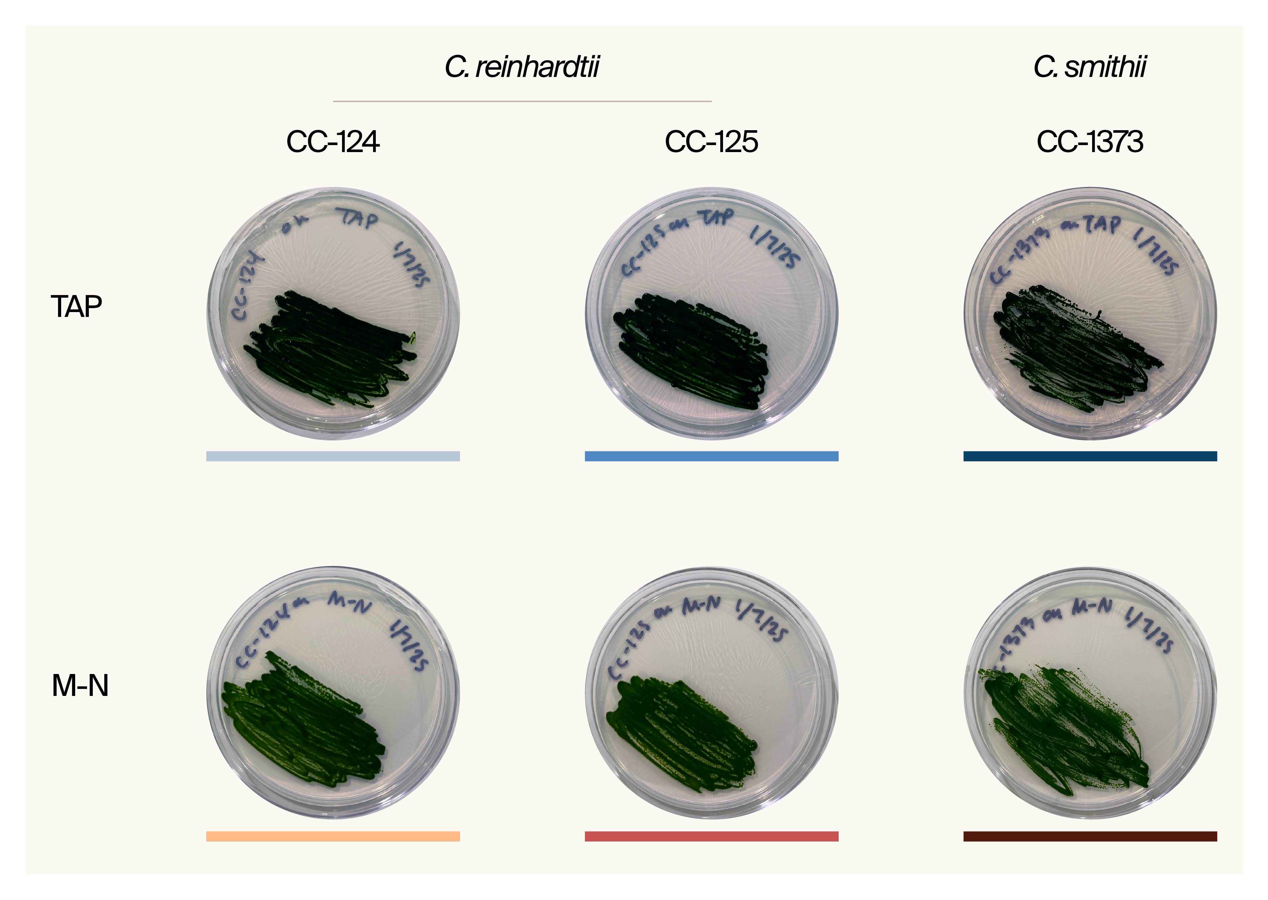
We compared three wild-type strains of Chlamydomonas grown on two types of solid media for a total of six treatments. There were two strains of Chlamydomonas reinhardtii, CC-124 (mating type -) and CC-125 (mating type +), and one strain of Chlamydomonas smithii, CC-1373 (mating type +).

Media components

We made all solid media with 1.5% agar. We made “water” plates with ultrapure water from a Milli-Q EQ 7008 system equipped with a 0.22 μm filter. Individual media components are as follows:

TAP (tris-acetate-phosphate) media
We purchased complete liquid media from UTEX.
M-N (minimal media lacking nitrogen) media
Made in-house following the above protocol.

Protocols

We maintained cells on TAP or M-N media plates with 1.5% agar under a 12/12 h light-dark cycle¹ at ambient temperature for 5–15 days before use. Cells were densely streaked to cover about half of the plate, creating a lawn. To acquire spectra from cells, we focused the laser on the portion of the plate with cells. To acquire background spectra from media and agar, we focused the laser on the area without cells.

¹ Note that we didn’t account for the timing within the light phase of the cycle when measurements were taken.

An image depicting the layout of plates of *Chlamydomonas* cell cultures. — Layout of *Chlamydomonas* plates.

To prepare slides with cells for microscopy (this was done only for the Renishaw InVa Qontor), we drew a wax circle on a #1.5 glass coverslip to create a hydrophobic barrier for each sample, making six total. We pipetted 3 µL of either liquid TAP or M-N media within the wax circles, resulting in three coverslips with each media type. We then transferred a small number of cells to the liquid droplet using a clean pipette. After transfer, clumps of cells were removed with forceps, resulting in a more continuous distribution of cells in each droplet. We repeated this for each of the three strains. Then, using forceps, we flipped each coverslip, placed it onto an ethanol-cleaned glass slide, and sealed each edge with melted VALAP (1:1:1 mixture of Vaseline, lanolin, and paraffin wax) using a paintbrush.

Analysis & results

Characterizing spectral resolution with acetonitrile

We acquired and analyzed measurements of the same sample of acetonitrile on each instrument to assess system performance. By analyzing the spectra and comparing them to established references, we’re able to characterize each instrument’s approximate spectral resolution and accuracy (the accuracy of the observed peak positions with respect to reference peaks).

We’ll start by loading the acetonitrile spectrum from each instrument as well as the standard Raman peaks for acetonitrile (Shimanouchi, 1972). While five standard peaks are listed in the NIST database as medium, strong, or very strong, the peak at 2,999 cm^–1 can be hard to detect, particularly with 532 nm excitation. For this reason, we’ll only characterize the four most prominent peaks and fit each with a Voigt model² (a convolution of a Gaussian distribution with a Lorentzian distribution) with a window size of 25.

² A Voigt profile is commonly used in peak fitting applications within spectroscopy because it accurately models spectral line shapes by accounting for both Doppler broadening (Gaussian component, due to thermal motion) and Lorentzian broadening (from collisional or lifetime effects). This makes it ideal for fitting experimental spectra where multiple broadening mechanisms contribute to the observed peak shape.

from analysis.load_spectra import load_acetonitrile_spectra
from lmfit.models import VoigtModel
from ramanalysis.calibrate import ACETONITRILE_PEAKS_CM1

# Load acetonitrile spectra and their corresponding spectrometers
acetonitrile_spectra, acetonitrile_dataframe = load_acetonitrile_spectra()

# Set parameters for peak finding
num_peaks = 4
window_size = 25
wavenumber_range_cm1 = (750, 3100)

Figure 1 shows the results of the peak fitting. Because the quartz cuvette of acetonitrile yields relatively strong and clean spectra, very little preprocessing is applied to the spectra. If you expand the code cell below, you’ll see that the only preprocessing steps applied are cropping the spectra to the wavenumber range (750–3,100 cm^–1) and min-max normalization. Only the OpenRAMAN spectrum is smoothed via median filtering to suppress hot pixels and read noise from the detector.

Note

Another strategy to deal with hot pixels from our acquisition would have been to acquire and subtract a dark spectrum (a spectrum with the laser powered off) to capture only the detector’s fixed pattern noise.

Source code for this figure:

import numpy as np
import pandas as pd
import plotly.graph_objects as go
from analysis.plotting import darken, get_custom_colorpalette, get_default_plotly_layout
from plotly.subplots import make_subplots
from ramanalysis.peak_fitting import find_n_most_prominent_peaks

# Store peak fitting results
peak_fitting_records = []

# Create figure
color_palette = get_custom_colorpalette()
num_rows = acetonitrile_dataframe.groupby(["λ_nm"]).count()["instrument"].max().item()
num_cols = acetonitrile_dataframe["λ_nm"].nunique()
fig = make_subplots(
    rows=num_rows,
    cols=num_cols,
    shared_xaxes=True,
    shared_yaxes=True,
    horizontal_spacing=0.02,
    vertical_spacing=0.05,
    column_titles=["785 nm", "532 nm"],
)

# Map each (instrument, wavelength) combo to a subplot
subplot_indices = {  # (instrument, λ_nm) -> (col, row)
    ("horiba", 785): (1, 1),
    ("renishaw", 785): (1, 2),
    ("wasatch", 785): (1, 3),
    ("openraman", 532): (2, 2),
    ("wasatch", 532): (2, 3),
}

for i, dataframe_row in acetonitrile_dataframe.iterrows():
    # Get the raw spectrum and the instrument and wavelength with which it was recorded
    wavelength_nm = dataframe_row["λ_nm"]
    instrument = dataframe_row["instrument"]
    raw_spectrum = acetonitrile_spectra[i]
    subplot_col, subplot_row = subplot_indices[(instrument, wavelength_nm)]

    # Apply median filtering on OpenRAMAN data to filter out hot pixels from the detector
    if instrument == "openraman":
        raw_spectrum = raw_spectrum.smooth(kernel_size=3)
    # Crop and normalize spectra for peak detection
    preprocessed_spectrum = raw_spectrum.between(*wavenumber_range_cm1).normalize()

    # Plot each acetonitrile spectrum
    name = f"{instrument.capitalize()}" if instrument != "openraman" else "OpenRAMAN"
    fig.add_trace(
        go.Scatter(
            x=preprocessed_spectrum.wavenumbers_cm1,
            y=preprocessed_spectrum.intensities,
            name=name,
            hoverinfo="skip",
            marker={"color": color_palette[(instrument, wavelength_nm)]},
        ),
        row=subplot_row,
        col=subplot_col,
    )

    # Find and get the indices of the most prominent peaks in the spectrum
    peak_indices = find_n_most_prominent_peaks(
        preprocessed_spectrum.intensities, num_peaks=num_peaks
    )
    for i_peak in peak_indices:
        # Create window around each peak
        peak_cm1, peak_height = preprocessed_spectrum.interpolate(i_peak)
        window_range = (i_peak - window_size / 2, i_peak + window_size / 2)
        window = np.linspace(*window_range, num=500)
        # Interpolate the window along the spectrum
        x_data_cm1, y_data = preprocessed_spectrum.interpolate(window)

        # Fit the model to each peak
        model = VoigtModel()
        initial_fit_params = model.make_params(amplitude=1, center=peak_cm1, sigma=1, gamma=0.5)
        fit_result = model.fit(y_data, initial_fit_params, x=x_data_cm1)

        # Find the offset from acetonitrile reference peaks
        peak_center = fit_result.params["center"].value
        reference_peak_index = np.abs(ACETONITRILE_PEAKS_CM1 - peak_center).argmin()
        reference_peak = ACETONITRILE_PEAKS_CM1[reference_peak_index]
        offset = peak_center - reference_peak

        # Record the peak fitting results
        peak_fitting_results = {**dataframe_row.to_dict(), **fit_result.params.valuesdict()}
        peak_fitting_results["reference"] = reference_peak
        peak_fitting_results["offset"] = offset
        peak_fitting_records.append(peak_fitting_results)

        # Plot and annotate each peak
        annotation_text = f"{peak_fitting_results['fwhm']:.1f} cm<sup>-1</sup>"
        hovertext_fields = ["fwhm", "height", "offset"]
        hovertext = [
            f"{field}: {peak_fitting_results[field]:.3g}<br>" for field in hovertext_fields
        ]
        fig.add_trace(
            go.Scatter(
                x=[peak_center],
                y=[peak_fitting_results["height"]],
                showlegend=False,
                hovertext="".join(hovertext),
                text=annotation_text,
                mode="markers+text",
                textposition="top center",
                marker={"color": darken(color_palette[(instrument, wavelength_nm)])},
            ),
            row=subplot_row,
            col=subplot_col,
        )

        # Plot fitted Voigt profile for each peak
        x_data = np.linspace(peak_center - window_size, peak_center + window_size, 500)
        model_params = [peak_fitting_results[p] for p in ["amplitude", "center", "sigma", "gamma"]]
        y_data = model.func(x_data, *model_params)
        fig.add_trace(
            go.Scatter(
                x=x_data,
                y=y_data,
                showlegend=False,
                hoverinfo="skip",
                marker={"color": darken(color_palette[(instrument, wavelength_nm)])},
            ),
            row=subplot_row,
            col=subplot_col,
        )

# Create pandas DataFrame of peak fitting results
acetonitrile_peaks_dataframe = pd.DataFrame.from_records(peak_fitting_records).drop("gamma", axis=1)

# Configure plotly layout
layout = get_default_plotly_layout()
fig.update_layout(layout, height=450)
fig.update_xaxes(range=[wavenumber_range_cm1[0] - 100, wavenumber_range_cm1[1] + 100])
fig.update_yaxes(range=[-0.05, 1.3])
fig.update_xaxes(title_text="Wavenumber (cm<sup>-1</sup>)", row=num_rows, col=1)
fig.update_xaxes(title_text="Wavenumber (cm<sup>-1</sup>)", row=num_rows, col=2)
fig.update_yaxes(title_text="Intensity (normalized)", row=2, col=1)
fig.show()

Figure 1: Acetonitrile spectra from each instrument. The four most prominent peaks for each spectrum are detected and fit using a Voigt profile. Hovering the cursor over each peak lets you see the measured FWHM, height, and offset from the reference peak value.

By analyzing the same acetonitrile sample across instruments, we can control for sample-dependent variables, allowing us to make meaningful comparisons of the relative performance of each spectrometer based on full width at half maximum (FWHM)³ measurements. The reference peak at ~918 cm^–1 is comparatively isolated, so the FWHM won’t be impacted by other components of the spectrum. Let’s choose this peak to compare FWHM values, noting that the observed FWHM is influenced by both instrumental factors (e.g., quality of optical components) and sample characteristics (e.g., molecular dynamics and environmental conditions).

³ While the FWHM serves as a useful indicator of spectral quality, it’s important to note that true spectral resolution is defined by the minimum separation at which two adjacent peaks can be distinguished rather than by individual peak widths alone.

acetonitrile_peaks_dataframe.query("reference == 918").set_index(["instrument", "λ_nm"]).round(1)

		amplitude	center	sigma	fwhm	height	reference	offset
instrument	λ_nm
horiba	785	10.9	918.5	4.7	11.7	0.8	918	0.5
renishaw	785	6.2	921.8	3.2	8.2	0.7	918	3.8
wasatch	785	6.5	921.4	4.8	11.9	0.5	918	3.4
openraman	532	4.0	921.4	8.7	21.0	0.2	918	3.4
wasatch	532	1.9	927.1	5.9	14.5	0.1	918	9.1

Table 1: Peak fitting results from acetonitrile spectra collected by each instrument.

The peak fitting results in Table 1 show that the Renishaw has the lowest FWHM of any instrument at 8.2 cm^-1. The Horiba and the 785 nm Wasatch are close behind at 11.7 cm^-1 and 11.9 cm^-1, respectively. Additionally, we found that the Horiba is the best calibrated in this spectral range as it has the smallest offset in peak position from the reference. While spectral accuracy is important, we’re less concerned here, given that we can always recalibrate spectra as part of a post-processing workflow using reference materials. Furthermore, for most of our research, we’re more interested in relative differences among spectra than absolute differences.

Let’s continue the comparison by exploring spectra from biological samples.

Characterizing SNR with C. reinhardtii spectra

We’re shifting our focus from a standard sample (acetonitrile) to biological samples, specifically unicellular algae, to determine how the different spectrometers perform for our experiments of interest. We collected Raman spectra of Chlamydomonas reinhardtii (CC-124) — a model organism we frequently use in the lab — from each instrument. Since biological samples introduce more complexity than pure compounds, we need to assess the signal-to-noise ratio (SNR) of these spectra to determine which instruments offer the highest sensitivity and are best suited for detecting subtle spectral features. This characterization will help us identify the most sensitive spectrometer for future experiments where detecting faint biochemical signals is critical. In addition to SNR measurements, we’ll make (relatively crude) peak-finding calculations to get a rough sense of the number of features we can resolve from each spectrum. We’ll use the find_peaks function from SciPy, which finds the local maxima in a 1D signal, and filter this set of local maxima to the peaks we’re interested in resolving by defining parameters such as the relative prominence and the distance between peaks.

We’ll also need to perform baseline subtraction to derive meaningful SNR measurements, as raw Raman spectra often contain fluorescence and other background signals that obscure meaningful peaks. In a separate analysis, we evaluated different baseline estimation algorithms. We found that adaptive smoothness penalized least squares (asPLS) performed the best at removing background while preserving key spectral features (Zhang et al., 2020). We use the implementation of asPLS in pybaselines with the smoothing parameter changed to lam = 1e4, as we found empirically that this value provided better baseline estimation for our dataset.

from analysis.load_spectra import load_cc124_tap_spectra
from pybaselines.whittaker import aspls
from ramanalysis import RamanSpectrum
from scipy.signal import find_peaks

cc124_tap_spectra, cc124_tap_dataframe = load_cc124_tap_spectra()


# Define a function for calculating peak SNR
def compute_peak_snr(
    spectrum: RamanSpectrum,
    noisy_region_cm1: tuple[float, float],
) -> float:
    """Peak SNR measurement."""
    noise = spectrum.normalize().between(*noisy_region_cm1).intensities.std()
    peak_snr = 1 / noise
    return peak_snr


# Parameters for baseline subtraction
lam = 1e4
wavenumber_range_cm1 = (520, 3200)

# Parameters for SNR calculation
noisy_region_cm1 = (1700, 2500)

# Parameters for peak finding
relative_prominences = {
    ("horiba", 785): 0.5,
    ("renishaw", 785): 0.1,
    ("wasatch", 785): 0.1,
    ("openraman", 532): 0.5,
    ("wasatch", 532): 0.1,
}
peak_separation = 10

Figure 2 shows the peak SNR measurements of each instrument and the approximate number of peaks.

Source code for this figure:

# Store peak SNR measurement results
snr_measurements = []

# Create figure
num_rows = cc124_tap_dataframe.groupby(["λ_nm"]).count()["instrument"].max().item()
num_cols = cc124_tap_dataframe["λ_nm"].nunique()
fig = make_subplots(
    rows=num_rows,
    cols=num_cols,
    shared_xaxes=True,
    shared_yaxes=True,
    horizontal_spacing=0.02,
    vertical_spacing=0.05,
    column_titles=["785 nm", "532 nm"],
)

# Map each (instrument, wavelength) combo to a subplot
subplot_indices = {  # (instrument, λ_nm) -> (col, row)
    ("horiba", 785): (1, 1),
    ("renishaw", 785): (1, 2),
    ("wasatch", 785): (1, 3),
    ("openraman", 532): (2, 2),
    ("wasatch", 532): (2, 3),
}

for i, dataframe_row in cc124_tap_dataframe.iterrows():
    # Get the raw spectrum and the instrument and wavelength with which it was recorded
    wavelength_nm = dataframe_row["λ_nm"]
    instrument = dataframe_row["instrument"]
    raw_spectrum = cc124_tap_spectra[i]
    subplot_col, subplot_row = subplot_indices[(instrument, wavelength_nm)]

    # Crop and normalize spectra for baseline estimation
    normalized_spectrum = raw_spectrum.between(*wavenumber_range_cm1).normalize()
    # Apply median filtering on OpenRAMAN data to filter out hot pixels from the detector
    if instrument == "openraman":
        normalized_spectrum = normalized_spectrum.smooth(kernel_size=3)

    # Estimate and subtract baseline
    baseline_estimate, _params = aspls(normalized_spectrum.intensities, lam=lam)
    baseline_subtracted_intensities = normalized_spectrum.intensities - baseline_estimate
    baseline_subtracted_spectrum = RamanSpectrum(
        wavenumbers_cm1=normalized_spectrum.wavenumbers_cm1,
        intensities=baseline_subtracted_intensities,
    ).normalize()

    # Crop out saturated region from Wasatch 532 nm spectrum
    if (instrument == "wasatch") and (wavelength_nm == 532):
        baseline_subtracted_spectrum = baseline_subtracted_spectrum.between(0, 1800).normalize()

    # Calculate peak SNR
    snr = compute_peak_snr(baseline_subtracted_spectrum, noisy_region_cm1)
    snr_measurements.append(snr)

    # Find prominent peaks
    peaks, _peak_properties = find_peaks(
        baseline_subtracted_spectrum.intensities,
        relative_prominences[(instrument, wavelength_nm)],
        distance=peak_separation,
    )
    peaks_cm1, peak_heights = baseline_subtracted_spectrum.interpolate(peaks)

    # Plot each raw (normalized) spectrum
    fig.add_trace(
        go.Scatter(
            x=normalized_spectrum.wavenumbers_cm1,
            y=normalized_spectrum.intensities,
            hoverinfo="skip",
            showlegend=False,
            marker={"color": color_palette[(instrument, wavelength_nm)]},
            opacity=0.5,
        ),
        row=subplot_row,
        col=subplot_col,
    )

    # Plot each baseline estimate
    fig.add_trace(
        go.Scatter(
            x=normalized_spectrum.wavenumbers_cm1,
            y=baseline_estimate - 0.05,
            hoverinfo="skip",
            showlegend=False,
            marker={"color": darken(color_palette[(instrument, wavelength_nm)])},
            opacity=0.5,
        ),
        row=subplot_row,
        col=subplot_col,
    )

    # Plot baseline subtracted spectra
    name = f"{instrument.capitalize()}" if instrument != "openraman" else "OpenRAMAN"
    fig.add_trace(
        go.Scatter(
            x=baseline_subtracted_spectrum.wavenumbers_cm1,
            y=baseline_subtracted_spectrum.intensities,
            name=name,
            hoverinfo="skip",
            marker={"color": color_palette[(instrument, wavelength_nm)]},
        ),
        row=subplot_row,
        col=subplot_col,
    )

    # Plot peaks
    fig.add_trace(
        go.Scatter(
            x=peaks_cm1,
            y=peak_heights,
            name=name,
            mode="markers",
            marker={"color": color_palette[(instrument, wavelength_nm)]},
            showlegend=False,
        ),
        row=subplot_row,
        col=subplot_col,
    )

    # Plot SNR and num peaks annotation
    text = f"Peak SNR: {snr:.1f}<br>Num peaks: {peaks.size:.0f}"
    fig.add_trace(
        go.Scatter(
            x=[2000],
            y=[0.6],
            showlegend=False,
            text=text,
            mode="text",
            textposition="middle right",
            name=name,
        ),
        row=subplot_row,
        col=subplot_col,
    )

# Create pandas DataFrame of peak fitting results
cc124_tap_dataframe["snr"] = snr_measurements

# Configure plotly layout
fig.update_layout(layout, height=450)
fig.update_xaxes(range=[wavenumber_range_cm1[0] - 100, wavenumber_range_cm1[1] + 100])
fig.update_yaxes(range=[-0.05, 1.3])
fig.update_xaxes(title_text="Wavenumber (cm<sup>-1</sup>)", row=num_rows, col=1)
fig.update_xaxes(title_text="Wavenumber (cm<sup>-1</sup>)", row=num_rows, col=2)
fig.update_yaxes(title_text="Intensity (normalized)", row=2, col=1)
fig.show()

Figure 2: Peak SNR measurements and detected peaks in C. reinhardtii spectra from each instrument. Each subplot shows the baseline-subtracted spectrum on which the peak SNR measurements are made. Behind the baseline-subtracted spectra, the raw C. reinhardtii spectra and estimated baselines are shown with semi-transparency. Note that the estimated baselines are slightly recessed from the raw spectra for visualization. Clicking on the instrument name in the legend toggles the display of the baseline-subtracted spectra to view the raw spectrum and estimated baseline more easily.

These measurements indicate that the Renishaw and 785 nm Wasatch systems provide the highest peak SNR values. The OpenRAMAN exhibits the lowest SNR, which aligns with expectations given its relatively low-cost components. In particular, the OpenRAMAN has by far the weakest laser power of any system and likely the most read noise from the detector; in contrast to the other systems, the camera is not cooled. Perhaps not surprisingly, the two instruments with the highest SNR also have the highest number of discernible spectral features.

The excitation wavelength greatly affects the usable signal. While it also has a relatively high SNR, the number of features in the 532 nm Wasatch spectrum is much lower. This suggests that 532 nm may be less optimal for analyzing these particular types of samples. It should be noted that the number of peaks detected in each spectrum is only an approximation.

Now, we’ll move on to applications requiring large spectral datasets, such as batch processing and machine learning (ML) techniques. These approaches will help us evaluate the reproducibility of each instrument and assess their sensitivity to subtle variations in differentiating strains and growth conditions of our cell samples, for example.

Batch preprocessing of Chlamydomonas spectra

The C. reinhardtii spectra characterized above come from a much larger dataset of Chlamydomonas spectra. Three strains of Chlamydomonas, representing two species, were cultured in two different media conditions, as described in Section 3. With each instrument, we acquired Raman spectra from plates (or, in the case of the Renishaw, glass slides) of cells representing each of these six treatments.

Let’s load the full dataset of spectra and associated metadata — a random sample of metadata from ten spectra from this dataset is shown in Table 2.

from analysis.load_spectra import load_chlamy_spectra

# Load all the spectra of Chlamydomonas and the corresponding metadata
chlamy_spectra, chlamy_dataframe = load_chlamy_spectra()

# Show a sample of spectra metadata
print(f"Total number of Chlamydomonas spectra: {len(chlamy_dataframe)}")
chlamy_dataframe.sample(10, random_state=57).reset_index(drop=True)

Total number of Chlamydomonas spectra: 536

	instrument	λ_nm	species	strain	medium
0	renishaw	785	C. reinhardtii	CC-124	TAP
1	renishaw	785	C. reinhardtii	CC-125	TAP
2	wasatch	532	C. smithii	CC-1373	TAP
3	openraman	532	C. reinhardtii	CC-125	TAP
4	openraman	532	C. smithii	CC-1373	M-N
5	wasatch	532	C. smithii	CC-1373	TAP
6	wasatch	785	C. reinhardtii	CC-125	M-N
7	wasatch	785	C. reinhardtii	CC-124	M-N
8	openraman	532	C. reinhardtii	CC-125	M-N
9	wasatch	785	C. reinhardtii	CC-125	M-N

Table 2: Metadata corresponding to a random sample of ten spectra from the Chlamydomonas dataset comprised of spectra from each instrument.

Since these spectra capture biochemical variations between species and environmental influences, we aim to apply machine-learning techniques to distinguish between groups. However, before diving into the modeling, we need to perform batch preprocessing to correct for background fluorescence, noise from the detectors, and other experimental inconsistencies. This ensures that our spectral differences reflect biological variability (as much as possible) rather than artifacts from acquisition conditions, improving the reliability of our classification models. The preprocessing pipeline is comprised of the following steps:

Denoising: Smooth spectra with Savitzky-Golay filter.
Cropping: Crop spectra to the region of interest (300–1,800 cm^–1).
Baseline subtraction: Fit and remove the fluorescence baseline using the asPLS algorithm.
Normalization: Apply min-max normalization to scale the spectra for consistency across samples.

Because data acquired with the Renishaw instrument was collected from glass slides, we need to perform an additional background subtraction. Glass has a distinct Raman spectrum that overlaps with spectral regions of interest from our biological samples (Fikiet et al., 2020), requiring a separate correction to prevent it from confounding our analysis. Figure 3 shows the results of our preprocessing pipeline on the Chlamydomonas dataset.

Note

When we collected data on the Horiba instrument, our focus wasn’t on ML classification tasks, so we didn’t design the dataset with that goal in mind. As a result, we don’t have a sufficient number of samples to support meaningful classification analysis. Given these limitations, we excluded this dataset from our classification efforts.

Source code for this figure and the preprocessing pipeline:

from scipy.signal import savgol_filter

# Preprocessing parameters
savgol_window_length = 9
savgol_polynomial_order = 3
fingerprint_region_cm1 = (300, 1800)

# Load spectrum from Renishaw glass slide control
txt_filepath = "data/Renishaw_Qontor/glass_slide_background.txt"
glass_slide_control_spectrum = RamanSpectrum.from_renishaw_txtfile(txt_filepath)

# Store preprocessed spectra
preprocessed_chlamy_spectra = []

for i, dataframe_row in chlamy_dataframe.iterrows():
    # Get the raw spectrum and its associated metadata
    raw_spectrum = chlamy_spectra[i]
    wavelength_nm = dataframe_row["λ_nm"]
    instrument = dataframe_row["instrument"]
    strain = dataframe_row["strain"]
    medium = dataframe_row["medium"]

    # Preprocessing steps
    # -------------------
    # 0.5) Apply median filtering on OpenRAMAN data to filter out hot pixels from the detector
    if instrument == "openraman":
        raw_spectrum = raw_spectrum.smooth(kernel_size=3)
    # 1) Denoising
    smoothed_intensities = savgol_filter(
        raw_spectrum.intensities,
        window_length=savgol_window_length,
        polyorder=savgol_polynomial_order,
    )
    # 1.5) Glass slide background subtraction for the Renishaw
    if instrument == "renishaw":
        smoothed_intensities -= glass_slide_control_spectrum.intensities
    # 2) Crop spectral range to the fingerprint region
    cropped_spectrum = RamanSpectrum(
        wavenumbers_cm1=raw_spectrum.wavenumbers_cm1,
        intensities=smoothed_intensities,
    ).between(*fingerprint_region_cm1)
    # 2.5) Additional cropping for 532 nm Wasatch
    if (instrument == "wasatch") and (wavelength_nm == 532):
        cropped_spectrum = cropped_spectrum.between(0, 1700)
    # 3) Baseline subtraction
    baseline_estimate, _params = aspls(cropped_spectrum.intensities, lam=lam)
    baseline_subtracted_intensities = cropped_spectrum.intensities - baseline_estimate
    # 4) Compose into RamanSpectrum and normalize
    preprocessed_spectrum = RamanSpectrum(
        wavenumbers_cm1=cropped_spectrum.wavenumbers_cm1,
        intensities=baseline_subtracted_intensities,
    ).normalize()
    preprocessed_chlamy_spectra.append(preprocessed_spectrum)

# Create figure
num_rows = len(chlamy_dataframe.groupby(["instrument", "λ_nm"]).nunique()) + 1
num_cols = 2
fig = make_subplots(
    rows=num_rows,
    cols=num_cols,
    row_heights=[0.5, 0.5, 0.1, 0.5, 0.5],  # add space to separate 532 vs 785 subplots
    shared_xaxes=True,
    shared_yaxes=True,
    horizontal_spacing=0.02,
    vertical_spacing=0.05,
    column_titles=["Raw", "Preprocessed"],
)
# Map each (instrument, wavelength) combo to a subplot
subplot_rows = {  # (instrument, λ_nm) -> row
    ("renishaw", 785): 1,
    ("wasatch", 785): 2,
    ("openraman", 532): 4,
    ("wasatch", 532): 5,
}

for (instrument, wavelength_nm), dataframe_group in chlamy_dataframe.groupby(
    ["instrument", "λ_nm"]
):
    # Only show a sample of spectra to avoid rendering issues
    num_samples = min(50, len(dataframe_group))
    for i, dataframe_row in dataframe_group.sample(num_samples).iterrows():
        # Get the raw and preprocessed spectra and its associated metadata
        raw_spectrum = chlamy_spectra[i]
        preprocessed_spectrum = preprocessed_chlamy_spectra[i]
        strain = dataframe_row["strain"]
        medium = dataframe_row["medium"]
        subplot_row = subplot_rows[(instrument, wavelength_nm)]

        # Plot each raw spectrum
        fig.add_trace(
            go.Scatter(
                x=raw_spectrum.wavenumbers_cm1,
                y=raw_spectrum.normalize().intensities,
                hoverinfo="skip",
                legendgroup=strain + medium,
                showlegend=False,
                marker={"color": color_palette[(strain, medium)]},
                opacity=0.5,
            ),
            row=subplot_row,
            col=1,
        )

        # Plot each preprocessed spectrum
        fig.add_trace(
            go.Scatter(
                x=preprocessed_spectrum.wavenumbers_cm1,
                y=preprocessed_spectrum.intensities,
                hoverinfo="skip",
                legendgroup=strain + medium,
                showlegend=False,
                marker={"color": color_palette[(strain, medium)]},
                opacity=0.5,
            ),
            row=subplot_row,
            col=2,
        )

# Plot fake traces for legend
ordered_groups = [
    ("CC-124", "TAP"),
    ("CC-125", "TAP"),
    ("CC-1373", "TAP"),
    ("CC-124", "M-N"),
    ("CC-125", "M-N"),
    ("CC-1373", "M-N"),
]
for strain, medium in ordered_groups:
    fig.add_trace(
        go.Scatter(
            x=[None],
            y=[None],
            mode="lines",
            name=f"{strain} | {medium}",
            line={"color": color_palette[(strain, medium)], "width": 3},
            legendgroup=strain + medium,
            showlegend=True,
        )
    )

# Configure plotly layout
fig.update_layout(layout, height=600)
fig.update_xaxes(title_text="Wavenumber (cm<sup>-1</sup>)", row=num_rows, col=1)
fig.update_xaxes(title_text="Wavenumber (cm<sup>-1</sup>)", row=num_rows, col=2)
for (instrument, wavelength_nm), row in subplot_rows.items():
    title = f"{instrument.capitalize()}<br>{wavelength_nm} nm"
    fig.update_yaxes(title_text=title, row=row, col=1)
fig.show()