From black box to glass box: Making UMAP interpretable with exact feature contributions –

Purpose

UMAP is a ubiquitous tool for low-dimensional visualization of high-dimensional datasets. UMAP learns a low-dimensional mapping from the nearest-neighbor graph structure of a dataset, often producing visually distinct clusters of data that align with known labels (e.g., cell types in a gene expression dataset). While the learned relationship between the input features and the embedding positions can be useful, the nonlinear UMAP embedding function also makes it difficult to directly interpret the mapping in terms of the input features.

Here, we show how to enable interpretation of the nonlinear mapping through a modification of the parametric UMAP approach, which learns the embedding with a deep network that is locally linear (but still globally nonlinear) with respect to the input features. This allows for the computation of a set of exact feature contributions as linear weights that determine the embedding of each data point. By computing the exact feature contribution for each point in a dataset, we directly quantify which features are most responsible for forming each cluster in the embedding space. We explore the feature contributions for a gene expression dataset from this “glass-box” augmentation of UMAP and compare them with features found by differential expression.

Introduction

UMAP (Uniform Manifold Approximation and Projection) is a powerful tool for nonlinear dimensionality reduction (McInnes et al., 2018). Despite some critical appraisals focused on the use of relative distances over the nonlinear embedding space to generate hypotheses as well as the black-box nature of the nonlinear mapping (Chari and Pachter, 2023; Ng et al., 2023), UMAP remains popular in many fields. Here, we present an augmentation to conventional UMAP analysis that generates exact feature attributions for each point in the dataset.

Principal components analysis (PCA) is another popular method for dimensionality reduction, which finds an alternative linear representation of a dataset by determining orthogonal directions of maximal variance. Since the principal components are the linear weights on input features, this approach is directly interpretable in feature space.

The recent popularity of UMAP comes at the cost of interpretable embeddings due to its nonlinearity. While nonlinear methods are generally thought to be black boxes, there are a range of post-hoc feature attribution methods that provide some measure of interpretability (like differential expression applied for gene expression data using ScanPy (v1.11.4) (Wolf et al., 2018) as well as GradCAM (Selvaraju et al., 2017) for image data). UMAP is popular due to its ability to successfully cluster classes for complex datasets in an unsupervised manner, despite its black-box nature.

UMAP generates distinct clusters as a black box, while PCA provides (sometimes less distinct) clusters for complex datasets, but also provides exact feature contributions. What if we could have the best of both approaches? A technique for interpreting nonlinear deep networks (Mohan et al., 2019; Wang et al., 2016) provides the key for bringing exact feature interpretability to UMAP.

Method

UMAP embeds high-dimensional data into a low-dimensional representation by building a nearest-neighbor graph in the original space and directly learning a set of embeddings in the representation space that best preserves local and global components of the nearest-neighbor graph according to a loss function.

The extension to a “parametric” form of UMAP (Pascarelli, 2023; Sainburg et al., 2021), where a deep network learns a function to generate a low-dimensional mapping, is a valuable generalization of the embedding approach, allowing new data points to be quickly embedded using the same mapping function. The deep network is trained using the same loss as the non-parametric model, so the network function captures the same relationships as the original non-parametric implementation.

The deep network approach for parametric UMAP is conventionally considered to be opaque to feature attribution. However, by leveraging a growing body of work in this area, we can implement a deep network with a specific architecture that enables us to measure the exact contributions of each input feature.

In Wang et al. (2016), Mohan et al. (2019) and Elhage et al. (2021), it is demonstrated that deep networks with zero-bias linear layers and specific types of activation functions possess exactly equivalent linear mappings. Even though these networks are globally nonlinear, which is why deep networks can learn such complex mappings, they are also locally linear or “point-wise” linear for a particular input (Golden, 2025). These networks fall into the category of homogeneous functions of order 1, which, based on Euler’s theorem, means a function has an equivalent representation with the Jacobian J which varies as a function of x:

y(x) = J(x) \cdot x \tag{1}

This mapping is linear and exact, although the Jacobian must be numerically computed for each input. Linear representations offer a straightforward approach to understanding what the network is computing. They are more interpretable than locally nonlinear networks (which include any deep network with nonzero bias terms in its linear layers).

It is straightforward to compute these linear feature contributions for every point in a dataset with a GPU. These types of deep networks for genomics data are locally linear, and from an interpretability perspective, they are effectively globally linear. We can easily perform an exhaustive local analysis, where we compute the Jacobian (via autograd) for every point in a dataset. With globally linear systems, there is only one set of feature weights to analyze. However, with locally linear systems, there are as many Jacobians (feature weights) as data points, which adds an additional step to the analysis.

The exactness of this Jacobian approach is the centerpiece of its appeal. This local analysis is similar to SHAP (Lundberg and Lee, 2017), LIME (Ribeiro et al., 2016), and GradCAM (Selvaraju et al., 2017); however, these methods are approximations that may be incorrect for the actual nonlinear function. The Jacobian of a zero-bias ReLU deep network weights each feature linearly, quantifying how the globally nonlinear network uses those features to generate its output.

Here, we apply these deep networks with linear equivalents to UMAP. In many papers, UMAP is presented as an interesting visual representation of data, but it is not frequently used beyond that. Conventionally, differential expression is applied to various clusters to identify genes that are differentially expressed on average (which is distinct from the features used by UMAP). In contrast, with fully interpretable glass-box networks, we can compute the exact contribution of each gene to the position of every single cell shown in the UMAP embedding space. Now, the exact gene feature contributions can be directly extracted from the nonlinear UMAP function, rather than from differential expression, which only acts as a proxy for what UMAP has learned. Additionally, the Jacobian approach works equally as well for image or protein embedding representations, where tools like differential expression are not available.

Beyond the feature attributions for each point, these can be aggregated over categories (like Leiden cluster or cell type) to generate hypotheses about the gene features connected to phenotypes represented in the dataset (York and Mets, 2025). This can be done in a straightforward manner by computing the feature attributions for all points of a given cell type (or Leiden cluster) and measuring summary statistics, like the mean or the singular value decomposition of the feature contributions.

The use of glass-box deep networks for UMAP, therefore, provides clarity into what the UMAP embedding function has actually learned.

Loading the data and tools

For an example dataset, we will use the human bone marrow gene expression data of Luecken et al. (2021), which is the example dataset now included in ScanPy (v1.11.4).

import os
import anndata as ad
import numpy as np
import pandas as pd
from matplotlib import font_manager as fm, pyplot as plt

# Config
TRAIN = False 

N_FITS = 16
N_FITS_TO_LOAD = 1
N_PCS = 50
EPOCHS = 64
RANDOM_STATE = 42
GROUPBY_KEY = 'cell_type'
MODEL_PATH_PATTERN = "models/umap_{i}.pth"
SUMMARY_BASENAME = "saved_outputs/bmmc_features_rev"
BATCH_KEY = "Samplename"

summary_stats_file = f"{SUMMARY_BASENAME}_stats.csv"
summary_plot_file = f"{SUMMARY_BASENAME}_plot_data.npz"
summary_interactive_file = f"{SUMMARY_BASENAME}_interactive.csv"

import os
import subprocess
import scanpy as sc
import anndata as ad
import pandas as pd

def download_bone_marrow_data(
    url="ftp://ftp.ncbi.nlm.nih.gov/geo/series/GSE194nnn/GSE194122/suppl/GSE194122_openproblems_neurips2021_cite_BMMC_processed.h5ad.gz",
    filename="GSE194122_openproblems_neurips2021_cite_BMMC_processed.h5ad.gz"
) -> ad.AnnData:
    """
    Downloads, unzips, and loads the bone marrow dataset.
    """
    unzipped_filename = filename.replace(".gz", "")
    if not os.path.isfile(unzipped_filename):
        if not os.path.isfile(filename):
            subprocess.run(["wget", url, "--no-verbose"])
        subprocess.run(["gunzip", filename])
    
    return sc.read_h5ad(unzipped_filename)

def preprocess_adata(
    adata: ad.AnnData,
    min_genes: int = 100,
    min_cells: int = 3,
    n_top_genes: int = 2000,
    n_pcs: int = 50,
    batch_key: str = "Samplename",
    run_scrublet: bool = False
) -> ad.AnnData:
    """
    Runs the full scRNA-seq preprocessing pipeline on an AnnData object.

    Args:
        adata (ad.AnnData): The raw AnnData object.
        min_genes (int): Min genes for cell filtering.
        min_cells (int): Min cells for gene filtering.
        n_top_genes (int): Number of highly variable genes to select.
        n_pcs (int): Number of principal components to compute.
        batch_key (str): The key in .obs for batch correction (if any).
        run_scrublet (bool): Whether to run doublet detection.

    Returns:
        ad.AnnData: The processed AnnData object.
    """
    print("--- Starting Preprocessing ---")
    
    # 1. Initial setup and QC gene flagging
    adata.obs_names_make_unique()
    adata.var_names_make_unique()
    adata.var["mt"] = adata.var_names.str.startswith("MT-")
    adata.var["ribo"] = adata.var_names.str.startswith(("RPS", "RPL"))
    adata.var["hb"] = adata.var_names.str.contains("^HB[^(P)]")
    
    # 2. Calculate QC
    sc.pp.calculate_qc_metrics(adata, qc_vars=["mt", "ribo", "hb"], inplace=True, log1p=True)
    
    # 3. Remove QC genes
    genes_to_remove = adata.var["mt"] | adata.var["ribo"] 
    adata._inplace_subset_var(~genes_to_remove)
    
    # 4. Filter cells, genes, and detect doublets
    sc.pp.filter_cells(adata, min_genes=min_genes)
    sc.pp.filter_genes(adata, min_cells=min_cells)
    if run_scrublet: 
        sc.pp.scrublet(adata, batch_key=batch_key)
    
    # 5. Normalize and find HVGs
    adata.layers["counts"] = adata.X.copy()
    sc.pp.normalize_total(adata)
    sc.pp.log1p(adata)
    sc.pp.highly_variable_genes(adata, n_top_genes=n_top_genes, batch_key=batch_key)
    
    # 6. Run PCA
    sc.tl.pca(adata, n_comps=n_pcs, use_highly_variable=True)
    
    return adata

The preprocessing pipeline follows the standard procedure for the dataset in the ScanPy (v1.11.4) clustering tutorial. We take the extra step of filtering out the less common cell types to simplify visualizations and keep only the top 12.

def prepare_data(groupby_key: str = 'cell_type', n_pcs: int = 50, batch_key: str = "Samplename") -> ad.AnnData:
    """
    Loads, concatenates, and preprocesses the scRNA-seq data.
    """
    adata_raw = download_bone_marrow_data()
    adata_raw.var_names_make_unique()

    # Slice and concatenate data
    if groupby_key == 'cell_type':
        adata_subset1 = adata_raw[adata_raw.obs['Samplename'] == 'site1_donor1_cite', :].copy()
        adata_subset3 = adata_raw[adata_raw.obs['Samplename'] == 'site1_donor3_cite', :].copy()
        adata_filtered = ad.concat([adata_subset1, adata_subset3], label="donors")
    else:
        adata_filtered = adata_raw
        
    adata_filtered.obs_names_make_unique()

    # Run the preprocessing pipeline on ALL concatenated cells first
    adata_processed = preprocess_adata(
        adata_filtered,  # <-- Use the unfiltered data
        n_top_genes=2000,
        n_pcs=n_pcs,
        batch_key=batch_key
    )

    # Now, filter to the top cell types for your analysis

    if groupby_key == 'cell_type':
        top_cell_types = adata_processed.obs[groupby_key].value_counts().nlargest(12).index
        # This subset now contains the .obsm['X_pca'] that was calculated on ALL cells
        adata_final = adata_processed[adata_processed.obs[groupby_key].isin(top_cell_types)].copy()
    if groupby_key.lower() == 'cd4+_t_cell_type':  
        adata_subset1 = adata_processed[adata_processed.obs['cell_type'] == 'CD4+ T activated', :].copy()
        adata_subset3 = adata_processed[adata_processed.obs['cell_type'] == 'CD4+ T naive', :].copy()

        adata_t_cells = ad.concat([adata_subset1,adata_subset3], label="T_cell_type")

        adata_final = scp.preprocess_adata(
            adata_t_cells,
            n_top_genes=1000, # You can use fewer HVGs for a subset
            n_pcs=50,         # You need fewer PCs for a subset
            batch_key="Samplename"
        )

    return adata_final

adata_final = prepare_data(
        groupby_key=GROUPBY_KEY, 
        n_pcs=N_PCS, 
        batch_key=BATCH_KEY
    )

We will also load a set of tools including the “UMAP PyTorch” toolbox in addition to ScanPy (v1.11.4), and define a custom PyTorch (v2.9.0) network to learn an embedding.

We perform several independent UMAP fits to the data, starting from different random initializations, to generate error bars for the feature contributions.

import os
import sys
import torch
import torch.nn.functional as F
import numpy as np
import pandas as pd
from collections import defaultdict

# --- Import PUMAP submodule ---
# (Assuming 'external/umap_pytorch' is in the working directory)
SUBMODULE_RELATIVE_PATH = 'external/umap_pytorch' 
project_root = os.getcwd()
submodule_root = os.path.join(project_root, SUBMODULE_RELATIVE_PATH)
if submodule_root not in sys.path:
    sys.path.insert(0, submodule_root) 
try:
    from umap_pytorch.main import PUMAP
except ImportError:
    print(f"Error: Could not import PUMAP from {submodule_root}.")
    print("Please ensure the submodule exists and is initialized.")
    sys.exit(1)
# ------------------------------

class GlassBoxUMAP:
    """
    Encapsulates the parametric UMAP model fitting and feature attribution.
    
    This class follows a scikit-learn style API:
    1. Initialize with hyperparameters.
    2. Fit with pre-processed data (e.g., PCA).
    3. Compute attributions using PCA data, gene expression, and PCA components.
    """
    def __init__(self,
                 # PUMAP params
                 n_components: int = 2,
                 n_neighbors: int = 15, 
                 min_dist: float = 0.3, 
                 repulsion_strength: float = 3.0,
                 # Training params
                 n_fits: int = 1, 
                 epochs: int = 64, 
                 lr: float = 1e-4, 
                 batch_size: int = 2048, 
                 random_state: int = 12,
                 # Network params
                 input_size: int = 50,
                 hidden_size: int = 1024 + 128
                 ):
        """Initializes the model with all hyperparameters."""
        self.n_components = n_components
        self.n_neighbors, self.min_dist, self.repulsion_strength = n_neighbors, min_dist, repulsion_strength
        self.n_fits, self.epochs, self.lr, self.batch_size, self.random_state = n_fits, epochs, lr, batch_size, random_state
        self.input_size = input_size
        self.hidden_size = hidden_size
        
        self.models_ = []
        self.embeddings_ = []
        self.jacobians_ = []
        self.feature_contributions_ = []
        self.device_ = 'cuda' if torch.cuda.is_available() else 'cpu'

    def fit(self, X: np.ndarray, 
            load_models: bool = False, 
            load_n_fits: int = 1,
            save_models: bool = True,
            model_path_pattern: str = "models/umap_{i}.pth"):
        """
        Fits the Parametric UMAP model to the input data X.

        Args:
            X (np.ndarray): The input data (e.g., PCA embeddings), 
                            shape (n_samples, n_features).
            load_models (bool): If True, skips training and loads pre-trained
                                models from `model_path_pattern`.
            save_models (bool): If True, saves the trained model weights to
                                `model_path_pattern` after fitting.
            model_path_pattern (str): A string pattern for the model file paths.
        """
        self.train_data_ = torch.tensor(X, dtype=torch.float32)
        
        self.models_ = []
        self.embeddings_ = []

        for i in range(self.n_fits):
            set_global_seeds(2*self.random_state + i)
            network = deepReLUNet(
                input_size=self.input_size, 
                hidden_size=self.hidden_size,
                output_size=self.n_components
            )
            
            pumap_model = PUMAP(
                encoder=network, n_neighbors=self.n_neighbors, 
                min_dist=self.min_dist, random_state=self.random_state + i,
                lr=self.lr, epochs=0 if load_models else self.epochs, # Only 1 epoch if loading
                batch_size=self.batch_size, num_workers=8, num_gpus=1
            )

            # Train or load
            model_file = model_path_pattern.format(i=i)
            
            if load_models:
                if i < load_n_fits:                                
                    try:
                        # print(pumap_model.trainer)
                        # pumap_model.trainer.load_from_checkpoint('/home/ubuntu/james/glass-box-umap/lightning_logs/version_110/checkpoints/epoch=63-step=320.ckpt')
                        pumap_model.device = self.device_
                        pumap_model.encoder.to(self.device_)
                        # We must "fit" with 1 epoch to initialize the graph
                        pumap_model.fit(self.train_data_) 
                        pumap_model.encoder.load_state_dict(
                            torch.load(model_file, map_location=self.device_)
                        )
                        pumap_model.encoder.eval() 

                        self.models_.append(pumap_model)
                        embedding = pumap_model.transform(self.train_data_) 
                        self.embeddings_.append(embedding)

                    except FileNotFoundError:
                        print(f"Error: Model file not found at {model_file}")
                        raise
                    except Exception as e:
                        print(f"Error loading state dict for model {i}: {e}")
                        raise
                    
            else:
                pumap_model.fit(self.train_data_)

                if save_models:
                    os.makedirs(os.path.dirname(model_file), exist_ok=True)
                    torch.save(pumap_model.encoder.state_dict(), model_file)
            
                self.models_.append(pumap_model)
                embedding = pumap_model.transform(self.train_data_) 
                self.embeddings_.append(embedding)
            
        return self

    def transform(self, X: np.ndarray, fit_index: int = 0) -> np.ndarray:
        """
        Transforms new data X into the embedding space using a trained model.

        Args:
            X (np.ndarray): New data to transform.
            fit_index (int): Index of the model to use for transformation.

        Returns:
            np.ndarray: The UMAP embedding.
        """
        if not self.models_:
            raise RuntimeError("The model must be fitted before transforming.")
        if fit_index >= len(self.models_):
            raise IndexError("fit_index is out of bounds.")
        
        X_tensor = torch.tensor(X, dtype=torch.float32)
        return self.models_[fit_index].transform(X_tensor)

    def fit_transform(self, X: np.ndarray, **kwargs) -> np.ndarray:
        """
        Fits the model to X and returns the embedding of X.
        
        Args:
            X (np.ndarray): The input data (e.g., PCA embeddings).
            **kwargs: Additional arguments passed to self.fit().

        Returns:
            np.ndarray: The UMAP embedding for the first fit (fit_index=0).
        """
        self.fit(X, **kwargs)
        return self.embeddings_[0]

    def compute_attributions(self, 
                             X_centered_gene_expression: np.ndarray, 
                             pca_components: np.ndarray, 
                             jacobian_batch_size: int = 40):
        """
        Computes the Jacobian and projects it to the original gene space.

        Args:
            X_centered_gene_expression (np.ndarray): Mean-centered gene expression
                data, shape (n_samples, n_genes).
            pca_components (np.ndarray): The PCA loading matrix (e.g., adata.varm["PCs"]),
                shape (n_genes, n_pcs).
            jacobian_batch_size (int): Batch size for Jacobian calculation.
        """
        if not self.models_:
            raise RuntimeError("The model must be fitted before computing contributions.")
        if self.train_data_ is None:
             raise RuntimeError("self.train_data_ not set. Please call fit() first.")
        
        self.feature_contributions_ = []
        self.jacobians_ = []

        for i, model in enumerate(self.models_):
            encoder = model.encoder
            encoder.eval()
            
            # 1. Compute Jacobian in batches (in PCA space)
            num_samples = self.train_data_.shape[0]
            jacobians_pca_list = []
            for j in range(0, num_samples, jacobian_batch_size):
                data_batch = self.train_data_[j:j + jacobian_batch_size, :]
                
                jac_batch = torch.autograd.functional.jacobian(
                    encoder, data_batch, vectorize=True, strategy="reverse-mode"
                )
                # Un-fuse the vectorized diagonal output
                jac_batch_unfused = torch.einsum('bibj->bij', jac_batch)
                jacobians_pca_list.append(jac_batch_unfused.detach().cpu())

            jacobians_pca_tensor = torch.cat(jacobians_pca_list, dim=0)

            # 2. Project Jacobian from PCA space back to gene space
            # J_gene[i, emb, gene] = J_pca[i, emb, pc] * PCs[gene, pc]
            gene_space_jacobian = torch.einsum(
                'bij,kj->bik', 
                jacobians_pca_tensor, 
                torch.tensor(pca_components, dtype=torch.float32)
            )

            # 3. Weight by each cell's mean-centered gene expression
            feature_contributions = gene_space_jacobian.numpy() * X_centered_gene_expression[:, np.newaxis, :]
            
            # For memory efficiency
            feature_contributions = feature_contributions.astype('float16')
            
            self.feature_contributions_.append(feature_contributions)
            self.jacobians_.append(jacobians_pca_tensor)

        return self

    def get_feature_importance(self, 
                               adata: 'ad.AnnData', 
                               groupby: str,
                               gene_names: np.ndarray) -> pd.DataFrame:
        """
        Aggregates feature contributions by a specified group.

        Args:
            adata (ad.AnnData): The AnnData object, needed for .obs groupings.
            groupby (str): The column in adata.obs to group by (e.g., 'cell_type').
            gene_names (np.ndarray): An array of gene names.

        Returns:
            pd.DataFrame: A DataFrame with mean and SEM contributions for
                          each gene in each group.
        """
        if not self.feature_contributions_:
            raise RuntimeError("Must run compute_attributions() first.")

        all_run_jacobians = np.array(self.feature_contributions_)
        n_runs = all_run_jacobians.shape[0]
        all_groups = adata.obs[groupby].cat.categories
        
        summary_dfs = []
        for group in all_groups:
            is_group_mask = (adata.obs[groupby] == group).values
            if np.sum(is_group_mask) == 0:
                continue # Skip if group has no cells

            # Shape: (n_runs, n_cells_in_group, n_dims, n_genes)
            jacobians_for_group = all_run_jacobians[:, is_group_mask, :, :]
            
            # Calculate magnitudes (L2 norm across UMAP dims)
            # Shape: (n_runs, n_cells_in_group, n_genes)
            magnitudes = np.linalg.norm(jacobians_for_group, axis=2, ord=2)
            
            run_mean_contributions = []
            for run_idx in range(n_runs):
                run_mags = magnitudes[run_idx, :, :] # (n_cells, n_genes)
                
                # Normalize each cell by its own total contribution
                cell_sums = np.sum(run_mags, axis=1, keepdims=True)
                normalized_mags = run_mags / (cell_sums + 1e-9)

                # Get the mean contribution for each gene across cells *for this run*
                run_mean_contributions.append(np.mean(normalized_mags, axis=0))
            
            # Aggregate across all runs
            # Shape: (n_runs, n_genes)
            run_means_array = np.array(run_mean_contributions) 
            
            # Final stats across runs
            mean_contributions = np.mean(run_means_array, axis=0)
            sem_contributions = np.std(run_means_array, axis=0) / np.sqrt(n_runs)

            df = pd.DataFrame({
                'gene': gene_names, 
                'mean_contribution': mean_contributions,
                'sem_contribution': sem_contributions, 
                groupby: group
            })
            summary_dfs.append(df)
            
        return pd.concat(summary_dfs, ignore_index=True)


    def save_analysis_summary(self, 
                              adata: 'ad.AnnData', 
                              groupby: str,
                              basename: str = "analysis_summary"):
        """
        Saves all necessary data for offline plotting and analysis.
        
        Args:
            adata (ad.AnnData): The AnnData object, needed for .obs groupings
                                and gene names.
            groupby (str): The column in adata.obs to group by (e.g., 'cell_type').
            basename (str): The prefix for the three output files.
        """
        if (not self.feature_contributions_ or 
            not self.embeddings_ or 
            not self.jacobians_ or 
            self.train_data_ is None):
            raise RuntimeError("Must run fit() and compute_attributions() first.")

        # 1. Save population-level statistics
        stats_df = self.get_feature_importance(adata, groupby, adata.var_names.values)
        stats_filename = f"{basename}_stats.csv"
        stats_df.to_csv(stats_filename, index=False)

        # 2. Save plot data (NPZ)
        mean_vector_dict = {}
        all_groups = adata.obs[groupby].cat.categories
        for group in all_groups:
            is_group_mask = (adata.obs[groupby] == group).values
            mean_vector_dict[group] = np.mean(self.feature_contributions_[0][is_group_mask], axis=0)
            
        jacobxall_first_run = self.feature_contributions_[0]
        jacobian_magnitude = np.linalg.norm(jacobxall_first_run, axis=1)

        jacobian_0 = self.jacobians_[0]
        pca_data_0 = self.train_data_.squeeze().detach().cpu().numpy()
        reconstruction_0 = np.einsum('ijk,ik->ij', jacobian_0.numpy(), pca_data_0)

        plot_data_filename = f"{basename}_plot_data.npz"
        np.savez_compressed(
            plot_data_filename,
            embedding=self.embeddings_[0],
            group_labels=adata.obs[groupby].values,
            group_by_key=groupby, # Store the key name
            mean_jacobian_vectors=mean_vector_dict,
            jacobian_magnitude=jacobian_magnitude,
            gene_names=adata.var_names.values,
            jacobian_reconstruction=reconstruction_0  
        )

        # 3. Save interactive plot data
        interactive_df = self._prepare_plotly_df(
            adata, groupby=groupby, fit_index=0, top_n_genes=8
        )
        interactive_filename = f"{basename}_interactive.csv"
        interactive_df.to_csv(interactive_filename, index=False)

    def _prepare_plotly_df(self, 
                           adata: 'ad.AnnData', 
                           groupby: str, 
                           fit_index: int = 0, 
                           top_n_genes: int = 8) -> pd.DataFrame:
        """(Private) Prepares a DataFrame for interactive plotting."""
        embedding = self.embeddings_[fit_index]
        jacobxall = self.feature_contributions_[fit_index]
        
        df = pd.DataFrame(embedding, columns=['UMAP 0', 'UMAP 1'])
        df[groupby] = adata.obs[groupby].values

        # Calculate squared distance and find top contributing genes
        gene_dist_sq = jacobxall[:, 0, :]**2 + jacobxall[:, 1, :]**2
        genes = adata.var.index.values
        
        top_gene_indices = np.argsort(gene_dist_sq, axis=1)[:, ::-1][:, :top_n_genes]
        
        for i in range(top_n_genes):
            df[f'gene_{i}'] = genes[top_gene_indices[:, i]]
            
        return df

from torch import nn
class LayerNormDetached(nn.Module):
    '''
    A LayerNorm implementation where the variance calculation is detached from the
    computation graph during evaluation, potentially stabilizing training.
    '''
    def __init__(self, emb_dim: int):
        super().__init__()
        self.scale = nn.Parameter(torch.ones(emb_dim))

    def forward(self, x: torch.Tensor) -> torch.Tensor:
        '''Forward pass for LayerNormDetached.'''
        mean = x.mean(dim=-1, keepdim=True)
        # Detach variance calculation during evaluation
        if not self.training:
            var = x.clone().detach().var(dim=-1, keepdim=True, unbiased=False)
        else:
            var = x.var(dim=-1, keepdim=True, unbiased=False)

        norm_x = (x - mean) / torch.sqrt(var + 1e-12) # Added epsilon for stability
        return self.scale * norm_x

class deepReLUNet(nn.Module):
    """
    A deep neural network using PReLU activation and LayerNormDetached.
    """
    def __init__(self, input_size: int = 50, hidden_size: int = 256, output_size: int = 2):
        super().__init__()
        self.model = nn.Sequential(
            nn.Linear(input_size, hidden_size, bias=False), nn.PReLU(), LayerNormDetached(hidden_size),
            nn.Linear(hidden_size, hidden_size, bias=False), nn.PReLU(), LayerNormDetached(hidden_size),
            nn.Linear(hidden_size, hidden_size, bias=False), nn.PReLU(), LayerNormDetached(hidden_size),
            nn.Linear(hidden_size, hidden_size, bias=False), nn.PReLU(), LayerNormDetached(hidden_size),
            nn.Linear(hidden_size, hidden_size, bias=False), nn.PReLU(),
            nn.Linear(hidden_size, output_size, bias=False)
        )

    def forward(self, x: torch.Tensor) -> torch.Tensor:
        """Forward pass through the PReLU network."""
        return self.model(x)

import random
import random
import numpy as np
# You may also need: import pytorch_lightning as pl

def set_global_seeds(seed: int):
    """Sets global seeds for reproducibility."""
    np.random.seed(seed)
    random.seed(seed)
    torch.manual_seed(seed)
    if torch.cuda.is_available():
        torch.cuda.manual_seed_all(seed)
    # Optional: For the Pytorch Lightning trainer
    # pl.seed_everything(seed) 
    
    # You might also want deterministic algorithms
    torch.backends.cudnn.deterministic = True
    torch.backends.cudnn.benchmark = False

# === 2. Model Fitting ===
print("\n=== 2. Model Fitting ===")
reducer = GlassBoxUMAP(
    n_fits=N_FITS,
    epochs=EPOCHS if TRAIN else 0, 
    random_state=RANDOM_STATE,
    input_size=N_PCS
)

reducer.fit(
    adata_final.obsm['X_pca'],
    load_models=not TRAIN,
    load_n_fits=N_FITS_TO_LOAD,
    save_models=TRAIN,
    model_path_pattern=MODEL_PATH_PATTERN
)

UMAP of gene expression data

Here we show the embeddings from the convetional, non-parametric UMAP from ScanPy (v1.11.4) as well as the PyTorch (v2.9.0) version of parametric UMAP. For visualizations we use the Arcadia Pycolor toolbox (“Arcadia-pycolor,” 2025) (v0.6.5).

# pumap_plotting

import scanpy as sc
import anndata as ad
import pandas as pd
import numpy as np
import matplotlib as mpl
import matplotlib.pyplot as plt
import matplotlib.ticker as ticker
from adjustText import adjust_text
import plotly.express as px
import plotly.graph_objects as go
import arcadia_pycolor as apc

import logging
logging.getLogger("scanpy.runtime").setLevel(logging.ERROR) 

def setup_plotting_themes():
    """Sets up the plotting themes for matplotlib and plotly."""
    apc.mpl.setup()
    apc.plotly.setup()

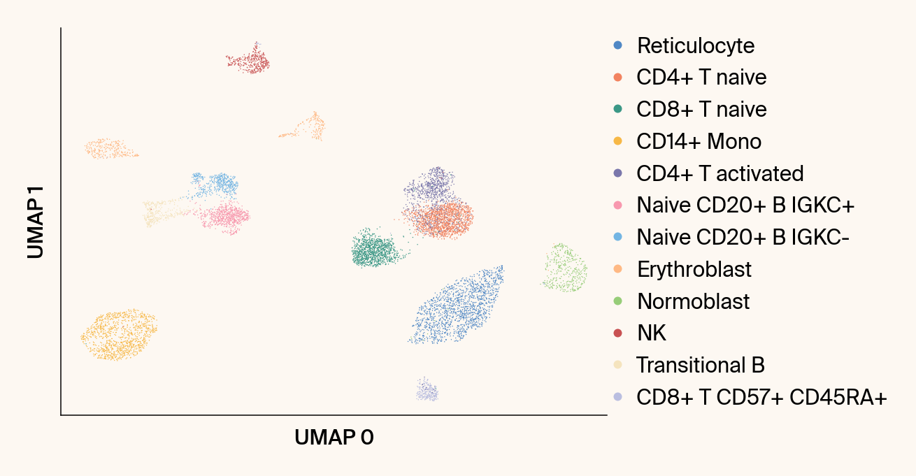
def plot_scanpy_umap(adata: ad.AnnData, 
                     groupby: str = 'cell_type', 
                     n_neighbors: int = 15, 
                     random_state: int = 13):
    """
    Computes and plots the standard non-parametric UMAP using Scanpy.
    
    Args:
        adata (ad.AnnData): The processed AnnData object.
        groupby (str): The .obs column to color by.
        n_neighbors (int): Number of neighbors for UMAP.
        random_state (int): Random state for UMAP.
    """
    
    if 'neighbors' not in adata.uns:
        sc.pp.neighbors(adata, n_neighbors=n_neighbors, use_rep='X_pca')
    
    # Compute standard UMAP
    sc.tl.umap(adata, init_pos='random', random_state=random_state)

    # Order categories by frequency
    category_order = adata.obs[groupby].value_counts().index.tolist()
    adata.obs[groupby] = adata.obs[groupby].astype('str').astype(
        pd.CategoricalDtype(categories=category_order, ordered=True)
    )

    with mpl.rc_context({"figure.facecolor": apc.parchment, "axes.facecolor": apc.parchment}):
        ax = sc.pl.umap(
            adata, color=groupby, size=2,
            palette=list(apc.palettes.primary), show=False
        )
        ax.set_xlabel("UMAP 0")
        ax.set_ylabel("UMAP 1")
        ax.spines['right'].set_visible(False)
        ax.spines['top'].set_visible(False)
        ax.set_title("")#f"{groupby} (Standard UMAP)")
        plt.show()

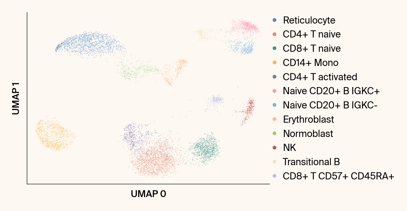
def plot_parametric_umap(reducer: GlassBoxUMAP, 
                         adata: ad.AnnData, 
                         fit_index: int = 0, 
                         groupby: str = 'cell_type'):
    """
    Plots the UMAP embedding from a specific parametric model fit.

    Args:
        reducer (GlassBoxUMAP): The fitted model object.
        adata (ad.AnnData): The processed AnnData object.
        fit_index (int): The index of the fitted model to visualize.
        groupby (str): The .obs column to color by.
    """
    if not reducer.embeddings_:
        raise RuntimeError("The reducer must be fitted before plotting.")
    
    resolved_index = fit_index if fit_index >= 0 else len(reducer.embeddings_) + fit_index

    # Order categories by frequency
    category_order = adata.obs[groupby].value_counts().index.tolist()
    adata.obs[groupby] = adata.obs[groupby].astype('str').astype(
        pd.CategoricalDtype(categories=category_order, ordered=True)
    )
        
    # Temporarily assign the parametric embedding to the default UMAP slot
    adata.obsm['X_umap'] = reducer.embeddings_[fit_index]

    with mpl.rc_context({"figure.facecolor": apc.parchment, "axes.facecolor": apc.parchment}):
        ax = sc.pl.umap(
            adata, use_raw=False, color=groupby, size=2,
            palette=list(apc.palettes.primary),
            show=False
        )
        ax.set_xlabel("UMAP 0")
        ax.set_ylabel("UMAP 1")
        ax.spines['right'].set_visible(False)
        ax.spines['top'].set_visible(False)
        ax.set_title("")#
        # ax.set_title(f"{groupby} (Parametric UMAP Fit {resolved_index})")
        plt.show()
            
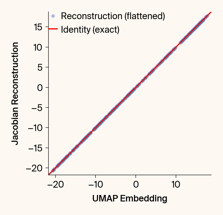
def validate_jacobian(
    reducer: 'GlassBoxUMAP', # Use quotes if class is not yet defined
    fit_index: int = 0, 
    n_samples: int = 100,
    dtype: torch.dtype = torch.float64
):
    """
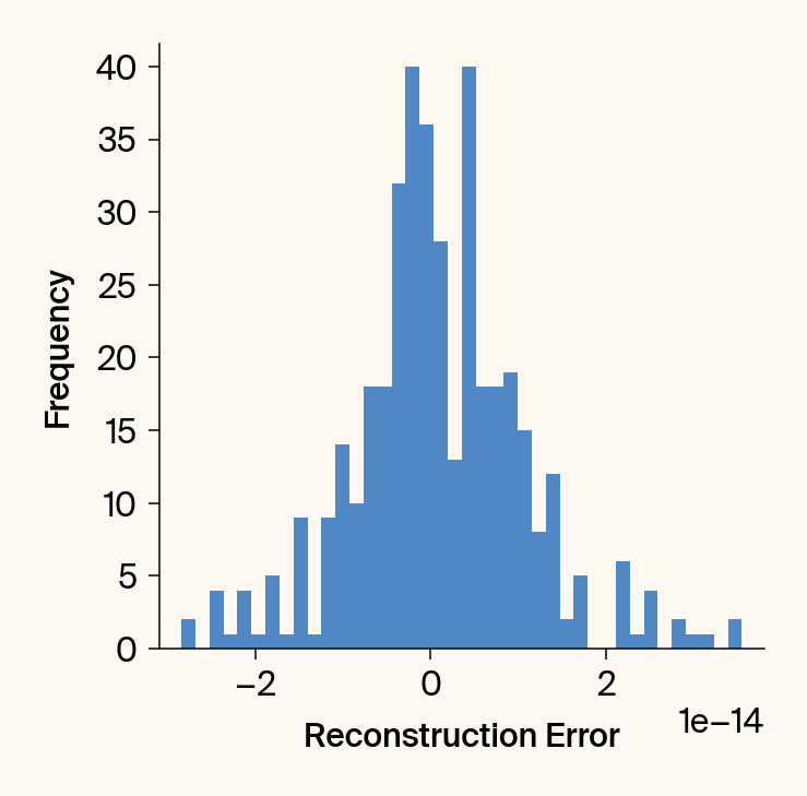
    Computes and plots the UMAP embedding vs. its reconstruction from the 
    on-the-fly Jacobian, and plots the reconstruction error.
    
    This function uses the computation method from your 'plot_error' example.
    
    Args:
        reducer (GlassBoxUMAP): The fitted model object.
        fit_index (int): The index of the fitted model to use.
        n_samples (int): The number of samples to use for the validation 
                         (from the start of the training set).
        dtype (torch.dtype): The dtype (e.g., torch.float64) for the computation.
    """
    
    if (not reducer.models_ or not reducer.train_data_ is not None):
        raise RuntimeError(
            "Must run fit() first to have models and training data available."
        )
    if fit_index >= len(reducer.models_):
        raise IndexError("fit_index is out of bounds for reducer.models_.")

    device = reducer.device_
    if "cuda" not in device:
        n_samples = 8
    
    encoder_casted = reducer.models_[fit_index].encoder.to(device=device, dtype=dtype)
    encoder_casted.eval()

    if n_samples > reducer.train_data_.shape[0]:
        n_samples = reducer.train_data_.shape[0]
        
    pca_data = reducer.train_data_[:n_samples]
    data_batch_casted = pca_data.to(device=device, dtype=dtype)
    
    jac_batch = torch.autograd.functional.jacobian(
        encoder_casted, data_batch_casted, vectorize=True, strategy="reverse-mode"
    )
    
    reconstruction = torch.einsum(
        'bibj,bj->bi', 
        jac_batch, 
        data_batch_casted
    )
    
    embedding = encoder_casted(data_batch_casted)
    
    err = reconstruction - embedding
    
    embedding_np = embedding.detach().cpu().numpy()
    reconstruction_np = reconstruction.detach().cpu().numpy()
    err_np = err.detach().cpu().numpy()

    try:
        plot_context = mpl.rc_context({
            "figure.facecolor": apc.parchment, 
            "axes.facecolor": apc.parchment
        })
    except Exception:
        print("Warning: 'apc.parchment' not found. Using default plot style.")
        plot_context = mpl.rc_context({}) 
    with plot_context:
        
        plt.figure()
        
        plt.scatter(embedding_np[:, :].flatten(), reconstruction_np[:, :].flatten(), alpha=0.5, label="Reconstruction (flattened)")
        
        global_min = min(embedding_np.min(), reconstruction_np.min())
        global_max = max(embedding_np.max(), reconstruction_np.max())
        
        # Add a small buffer
        min_val = global_min - 1
        max_val = global_max + 1
        plt.plot([min_val, max_val], [min_val, max_val], 'r', linewidth=2, label="Identity (exact)")

        plt.xlabel('UMAP Embedding')#, labelpad=33.8)
        plt.ylabel('Jacobian Reconstruction')
        plt.legend()            
        # plt.axis('square')
        plt.xlim(min_val, max_val)
        plt.ylim(min_val, max_val)
        ax1=plt.gca()
        # ax1.set_aspect('equal', adjustable='box')
        ax1.set_box_aspect(1)
        plt.show()

        plt.figure()
        plt.hist(err_np.flatten(), bins=40)
        # current_ax = plt.gca()
        # current_ax.xaxis.set_major_locator(plt.MaxNLocator(nbins=5, prune='both'))
        plt.xlabel('Reconstruction Error')# (Reconstruction - Embedding)', labelpad=20)
        plt.ylabel('Frequency')
        ax2=plt.gca()
        # ax2.set_aspect('equal', adjustable='box')
        ax2.set_box_aspect(1)
        # plt.title(f'Histogram of Reconstruction Error ({dtype})')
        plt.show()
        
def plot_interactive(
    reducer: GlassBoxUMAP,
    adata: ad.AnnData,
    groupby: str = 'cell_type',
    color_by: str = 'group', 
    top_n_to_show: int = 16, 
    show_centroids: bool = False, 
    fit_index: int = 0,
    summary_file: str = "analysis_summary_interactive.csv",
    show_percentage: bool = False
):
    """
    Generates an interactive Plotly UMAP embedding.
    
    Args:
        reducer (GlassBoxUMAP): The fitted model object.
        adata (ad.AnnData): The processed AnnData object.
        groupby (str): The .obs column to use for grouping (e.g., 'cell_type').
        color_by (str): 'group' (to color by `groupby` key) or 'top_gene'.
        summary_file (str): Path to the .csv file for loading/saving.
    """
    import os
    
    if summary_file and os.path.exists(summary_file):
        df = pd.read_csv(summary_file)

        if groupby not in df.columns:
            print(f"Warning: Column '{groupby}' not found in {summary_file}.")
            
            potential_cols = [col for col in df.columns if 
                              col not in ['UMAP 0', 'UMAP 1'] and 
                              not col.startswith('gene_')]
            
            if len(potential_cols) == 1:
                old_groupby = potential_cols[0]
                df = df.rename(columns={old_groupby: groupby})
            else:

                raise KeyError(
                    f"Column '{groupby}' not found in {summary_file}. "
                    f"Found potential group columns: {potential_cols}. "
                    "The summary file may be stale. "
                    "Try running with TRAIN=True to regenerate it."
                )

    else:
        if not reducer.feature_contributions_:
            raise RuntimeError("Must run compute_attributions() first to generate data.")
        
        df = reducer._prepare_plotly_df(adata, groupby, fit_index=fit_index)
        
        if summary_file:
            df.to_csv(summary_file, index=False)

    hover_data = ['gene_0', 'gene_1', 'gene_2', groupby]
    
    if color_by == 'group':
        fig = px.scatter(
            df, x='UMAP 0', y='UMAP 1', color=groupby,
            # title=f'Bone Marrow Gene Expression: {groupby}',
            hover_data={k: True for k in hover_data if k != groupby},
            category_orders={groupby: df[groupby].astype('category').value_counts().index},
            color_discrete_sequence=(apc.palettes.primary + apc.palettes.secondary)
        )
        grouping_col, data_for_centroids = groupby, df
    
    elif color_by == 'top_gene':
        df['gene_0'] = df['gene_0'].astype(str)
        top_genes = df['gene_0'].value_counts().nlargest(top_n_to_show).index
        df_filtered = df[df['gene_0'].isin(top_genes)]
        percent_shown = len(df_filtered) / len(df)
        # title = f'Bone Marrow: Top Gene Contributors, ({percent_shown:.1%} of cells shown)'
        fig = px.scatter(
            df_filtered, x='UMAP 0', y='UMAP 1', color='gene_0',
            title="", hover_data=hover_data,
            category_orders={'gene_0': top_genes},
            color_discrete_sequence=(apc.palettes.secondary + apc.palettes.primary)
        )
        grouping_col, data_for_centroids = 'gene_0', df_filtered
    
    else:
        raise ValueError("color_by must be 'group' or 'top_gene'")

    if show_centroids:
        centroids = data_for_centroids.groupby(grouping_col)[['UMAP 0', 'UMAP 1']].mean()
        for label, center in centroids.iterrows():
            fig.add_annotation(
                x=center['UMAP 0'], y=center['UMAP 1'], text=f"<b>{label}</b>",
                showarrow=False, font=dict(size=16, color='black'),
                align='center', bgcolor='rgba(255, 255, 255, 0.5)', borderpad=4
            )
            
    fig.update_traces(marker_size=3)
    fig.update_layout(
        autosize=True, 
        yaxis_scaleanchor="x",
        legend={'itemsizing': 'constant', 'y': 1, 'x': 1.0, 'yanchor': 'top', 'xanchor': 'left'}
    )

    apc.plotly.style_plot(fig, monospaced_axes="all")
    fig.show()
    if color_by == 'top_gene' and show_percentage:
        print(f'Bone Marrow: Top Gene Contributors, ({percent_shown:.1%} of cells shown)')

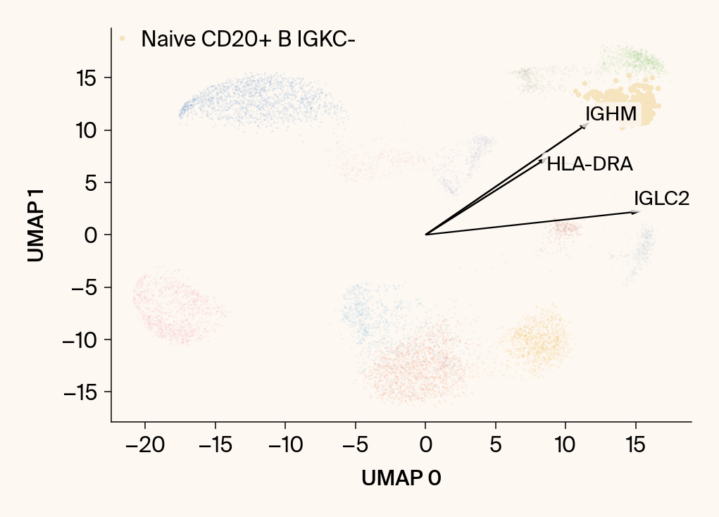
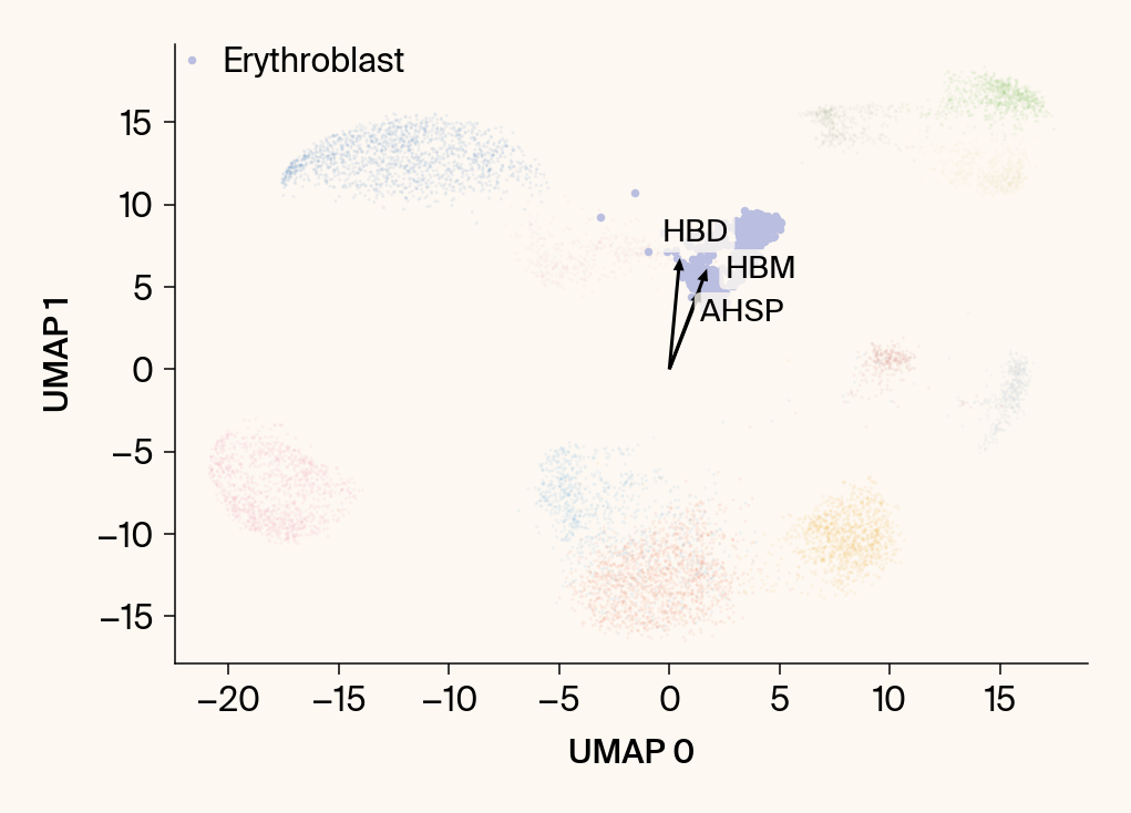
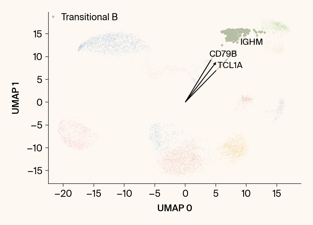
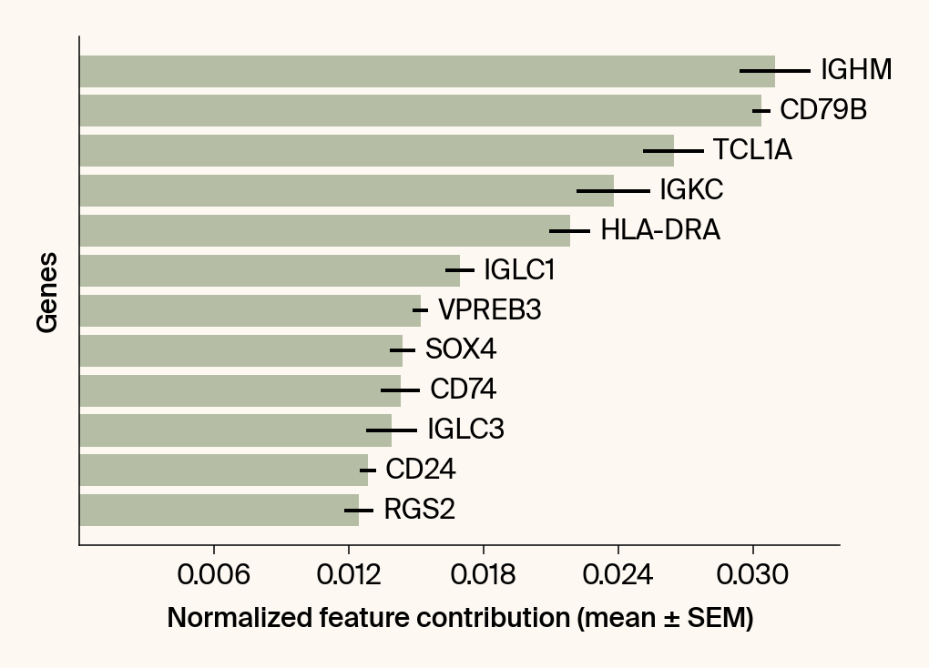
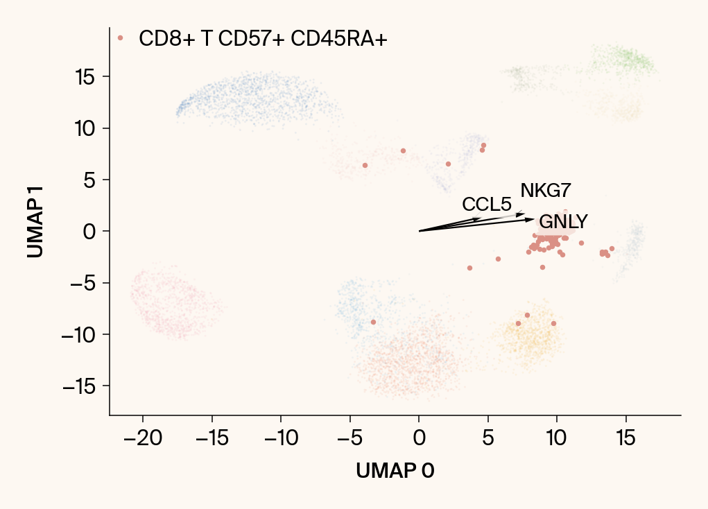
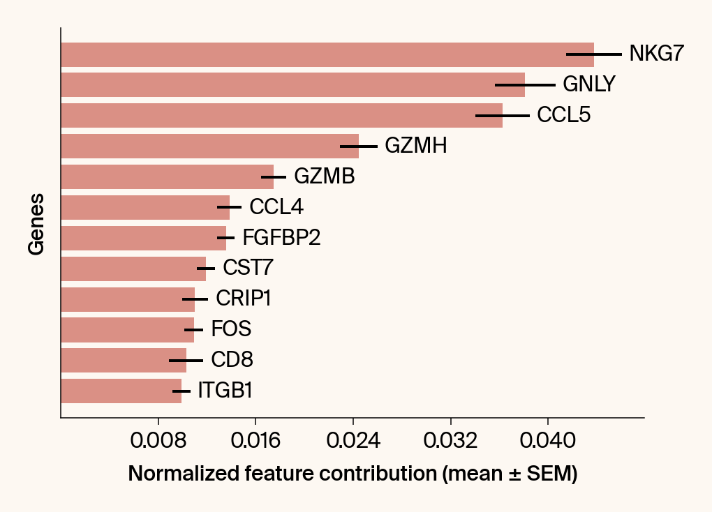
def plot_feature_importance_by_group(
    reducer: GlassBoxUMAP,
    adata: ad.AnnData,
    groupby: str = 'cell_type',
    n_features_bars: int = 12, 
    n_features_vectors: int = 3,
    fit_index: int = 0, 
    groups_to_plot: list = None,
    summary_stats_file: str = "analysis_summary_stats.csv",
    summary_plot_file: str = "analysis_summary_plot_data.npz",
    set_axes_equal: bool = False,
    plot_sum_features: bool = False
):
    """
    Analyzes and visualizes feature contributions for each group.
    
    Args:
        reducer (GlassBoxUMAP): The fitted model object.
        adata (ad.AnnData): The processed AnnData object.
        groupby (str): The .obs column to use for grouping (e.g., 'cell_type').
        groups_to_plot (list): A list of specific group names to plot. 
                               If None, plots the top 12.
    """
    import os
    # Add necessary imports that were implicit in the original
    import pandas as pd
    import numpy as np
    import matplotlib.pyplot as plt
    import matplotlib as mpl
    from adjustText import adjust_text
    # Assuming 'apc' is available in the environment (e.g., import anndata_plotting_context as apc)
    # Assuming 'ad' (anndata) is available
    
    can_load_from_file = (
        summary_stats_file and os.path.exists(summary_stats_file) and
        summary_plot_file and os.path.exists(summary_plot_file)
    )
    
    if can_load_from_file:
        summary_df = pd.read_csv(summary_stats_file)
        with np.load(summary_plot_file, allow_pickle=True) as data:
            embedding = data['embedding']
            
            try:
                group_labels_array = data['group_labels']
                loaded_groupby_key = str(data['group_by_key']) if 'group_by_key' in data else 'cell_type' 
            except KeyError:
                print("Warning: 'group_labels' key not found. Trying fallback 'cell_types'...")
                try:
                    group_labels_array = data['cell_types'] 
                    loaded_groupby_key = 'cell_type' 
                except KeyError:
                    raise KeyError(
                        "Could not find 'group_labels' or 'cell_types' in the .npz file. "
                        "The summary file may be stale or corrupt. "
                        "Try running with TRAIN=True to regenerate it."
                    )
            
            mean_jacobian_vectors = data['mean_jacobian_vectors'].item()
            gene_names_original_order = data['gene_names']
            
            if loaded_groupby_key != groupby:
                print(f"Warning: File was grouped by '{loaded_groupby_key}', "
                      f"but you requested '{groupby}'. Results may be incorrect.")
        
        all_groups = pd.Series(group_labels_array).value_counts().index
        
    else:
        if not reducer.feature_contributions_:
            raise RuntimeError("Must run compute_attributions() first to generate data.")
        
        embedding = reducer.embeddings_[fit_index]
        group_labels_array = adata.obs[groupby].values
        all_groups = adata.obs[groupby].value_counts().index
        gene_names_original_order = adata.var_names.values 
        
        summary_df = reducer.get_feature_importance(adata, groupby, gene_names_original_order)

        mean_jacobian_vectors = {}
        for group in all_groups:
            is_group_mask = (adata.obs[groupby] == group).values
            mean_jacobian_vectors[group] = np.mean(
                reducer.feature_contributions_[fit_index][is_group_mask], axis=0
            )

    if groups_to_plot is None:
        groups_to_plot = all_groups[:12]
    
    # This assumes 'apc' is an imported module available in the scope
    cmap = (apc.palettes.primary + apc.palettes.secondary).to_mpl_cmap()
    category_colors = [cmap(i / len(all_groups)) for i in range(len(all_groups))]
    color_map = {name: color for name, color in zip(all_groups, category_colors)}
    point_colors = np.array([color_map.get(ct, 'gray') for ct in group_labels_array])

    gene_to_original_index = {gene: i for i, gene in enumerate(gene_names_original_order)}

    with mpl.rc_context({"figure.facecolor": apc.parchment, "axes.facecolor": apc.parchment}):
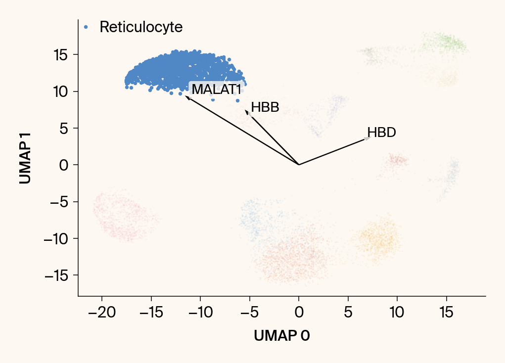
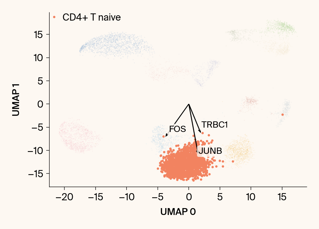
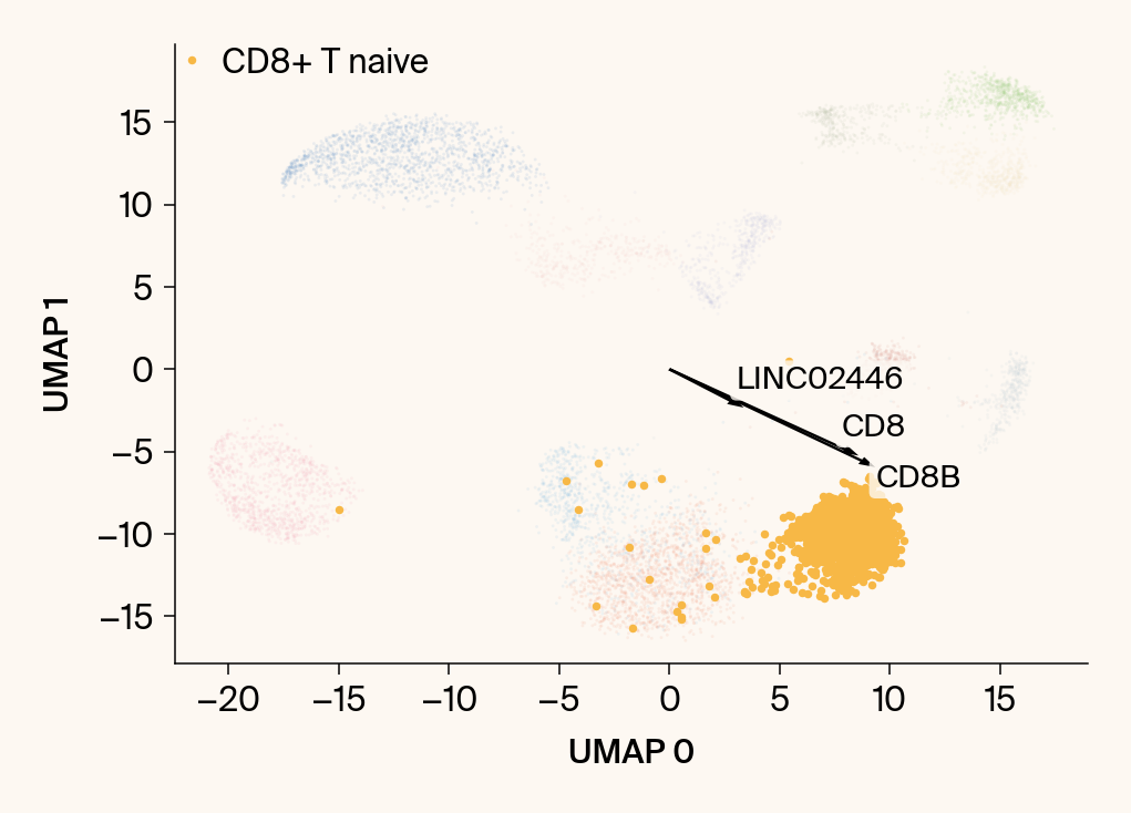
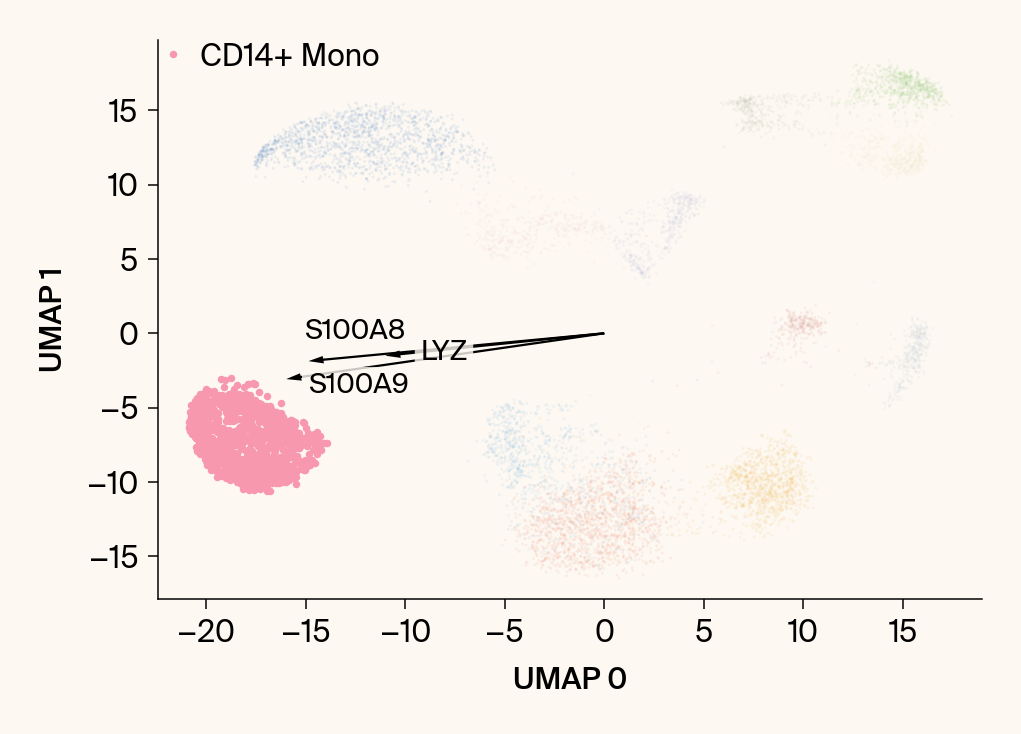
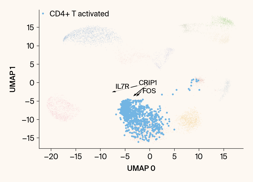
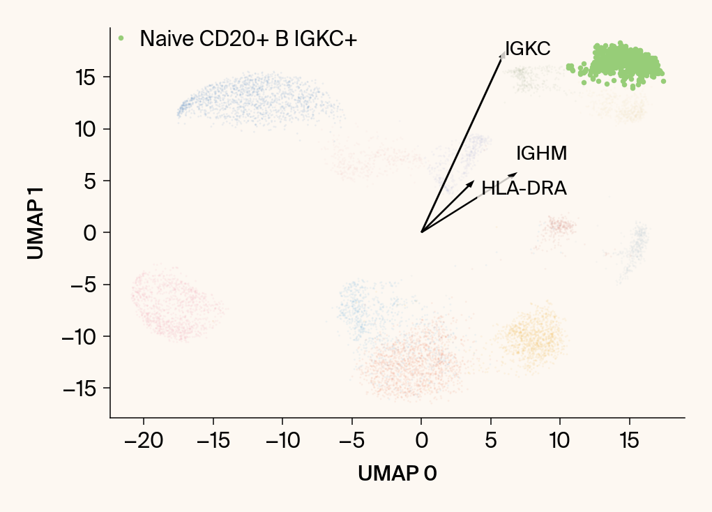
        for group in groups_to_plot:
            
            # --- Plot 1: Scatter plot with vectors ---
            
            # Create new figure without subplots
            fig1 = plt.figure()#figsize=[6, 6])
            
            is_group_mask = (group_labels_array == group)

            # Use plt. scatter, xlabel, ylabel, grid, legend
            plt.scatter(embedding[:, 0], embedding[:, 1], c=point_colors, s=2, alpha=0.1)
            plt.scatter(embedding[is_group_mask, 0], embedding[is_group_mask, 1], 
                        c=[color_map.get(group, 'gray')], s=14, marker="o", label=group)
            plt.xlabel("UMAP 0"); plt.ylabel("UMAP 1")
            plt.grid(False); plt.legend()
            
            # Get current axis for commands that require an axis object
            current_ax = plt.gca()
            current_ax.spines[['right', 'top']].set_visible(False)
            if set_axes_equal:
                current_ax.set_box_aspect(1)
            
            group_df = summary_df[summary_df[groupby] == group].sort_values('mean_contribution', ascending=False)
            
            if group_df.empty:
                print(f"Skipping plot for {group}: no data found in summary.")
                plt.close(fig1) # Close the empty figure
                continue

            top_bar_indices = group_df.index[:n_features_bars]
            top_vector_indices = group_df.index[:n_features_vectors]
            
            vectors_for_group = mean_jacobian_vectors.get(group)
            if vectors_for_group is None:
                print(f"Skipping vectors for {group}: no mean_jacobian_vectors found.")
                continue
            
            cluster_centroid = np.mean(embedding[is_group_mask], axis=0)
            
            top_gene_names = group_df.loc[top_vector_indices, 'gene']
            top_gene_original_indices = [gene_to_original_index[gene] for gene in top_gene_names if gene in gene_to_original_index]

            if top_gene_original_indices:
                max_vector_mag = np.max(np.linalg.norm(vectors_for_group[:, top_gene_original_indices], axis=0))
                scale_factor = (np.linalg.norm(cluster_centroid) / (max_vector_mag + 1e-6)) * 0.8
            else:
                scale_factor = 1.0

            texts = []
            for gene_idx in top_vector_indices:
                gene_name = group_df.loc[gene_idx, 'gene']
                gene_original_index = gene_to_original_index.get(gene_name)
                
                if gene_original_index is not None:
                    vec = vectors_for_group[:, gene_original_index] * scale_factor
                    # Use plt.arrow and plt.text
                    plt.arrow(0, 0, vec[0], vec[1], width=0.15, color='k', head_width=0.5, zorder=3)
                    texts.append(plt.text(vec[0], vec[1], gene_name, fontsize=14,
                                        bbox=dict(boxstyle="round,pad=0.2", fc=apc.parchment, ec="none", alpha=0.8)))
            
            if texts:
                # adjust_text requires an explicit axis
                adjust_text(texts, ax=current_ax, arrowprops=dict(arrowstyle="-", color='gray', lw=0.5))

            top_genes = group_df.loc[top_bar_indices, 'gene'][::-1]
            top_means = group_df.loc[top_bar_indices, 'mean_contribution'][::-1]
            top_sems = group_df.loc[top_bar_indices, 'sem_contribution'][::-1]
            
            if plot_sum_features:
                # Assuming n_features_vectors is at least 20, or you want the top 'n_features_vectors'
                # Change the index to top 20 features, or use the existing variable
                top_path_indices = group_df.index[:220]

                # --- Initialize starting point and list for line segments ---
                current_pos = np.array([0.0, 0.0])
                path_points = [current_pos.copy()] # Start the path at (0, 0)

                # --- Calculate the sequential path and plot vectors ---
                for gene_idx in top_path_indices:
                    gene_name = group_df.loc[gene_idx, 'gene']
                    gene_original_index = gene_to_original_index.get(gene_name)

                    if gene_original_index is not None:
                        
                        vec = vectors_for_group[:, gene_original_index] 
                        
                        # --- Plot the vector segment ---
                        # The vector starts at the end of the previous one (current_pos)
                        # and points to the new position (current_pos + vec)
                        plt.arrow(current_pos[0], current_pos[1], vec[0], vec[1], 
                                width=0.15, color='r', head_width=0.0, zorder=4, 
                                label='Sequential Path' if len(path_points) == 1 else None)
                        
                        # --- Update position and path points ---
                        current_pos += vec
                        path_points.append(current_pos.copy())
                        
                        # --- Add text label at the end of the vector segment ---
                        # plt.text(current_pos[0], current_pos[1], gene_name, fontsize=10, color='r',
                        #         bbox=dict(boxstyle="round,pad=0.1", fc='white', ec="none", alpha=0.6))

                # --- Plot the path as a single line for clarity (optional) ---
                path_points_array = np.array(path_points)
                plt.plot(path_points_array[:, 0], path_points_array[:, 1], 'r--', alpha=0.5, zorder=3)

            fig1.tight_layout()
            plt.show()
            
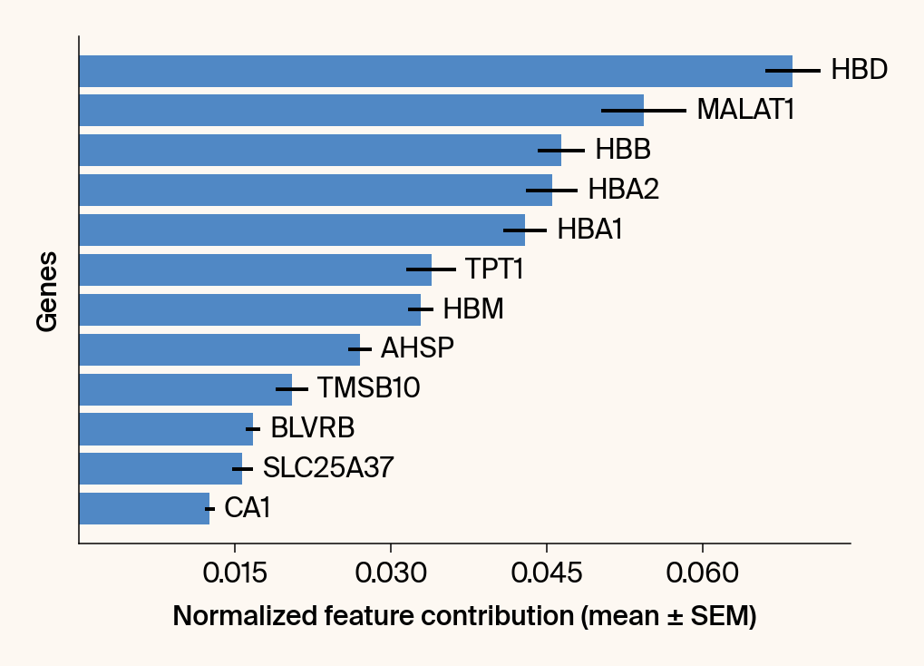
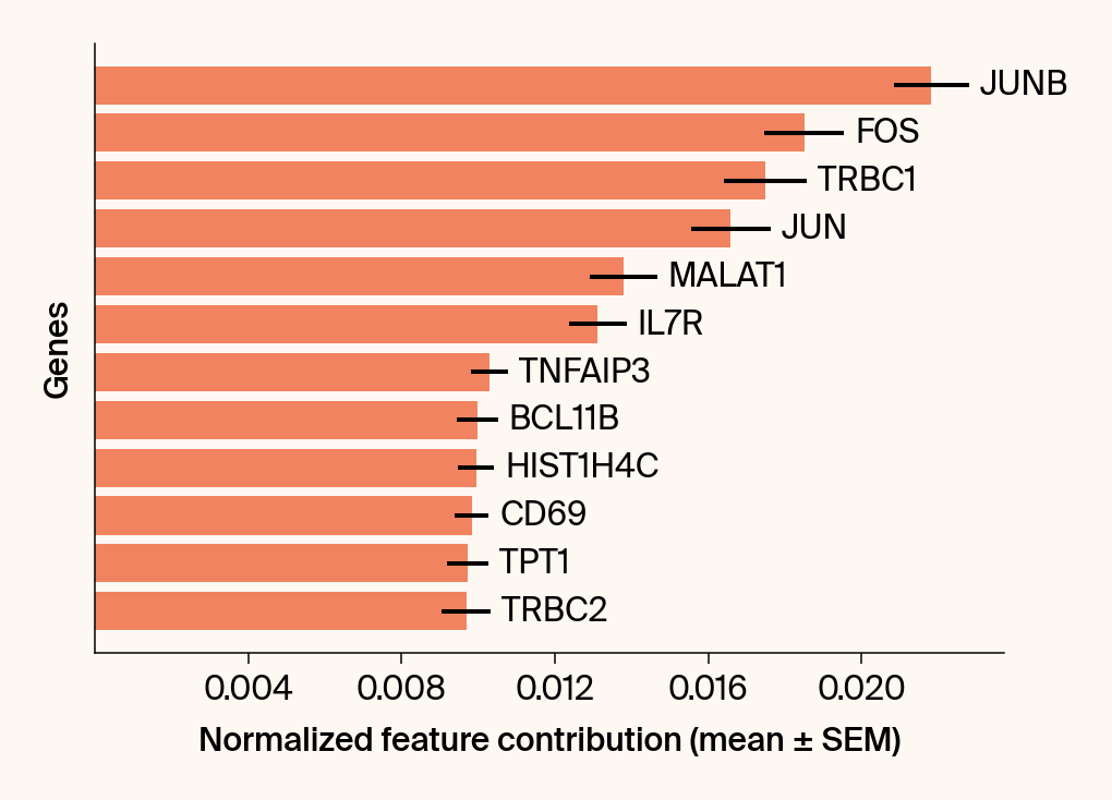
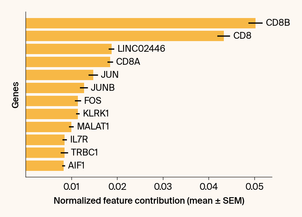
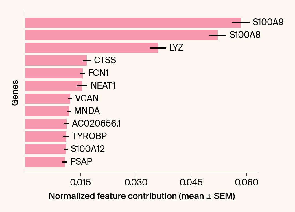
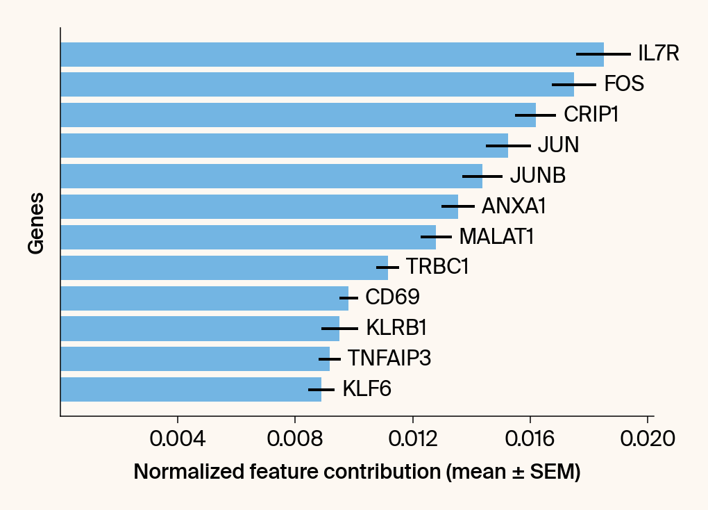
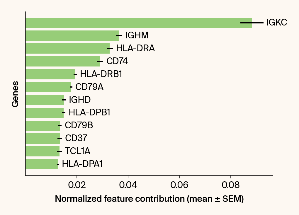
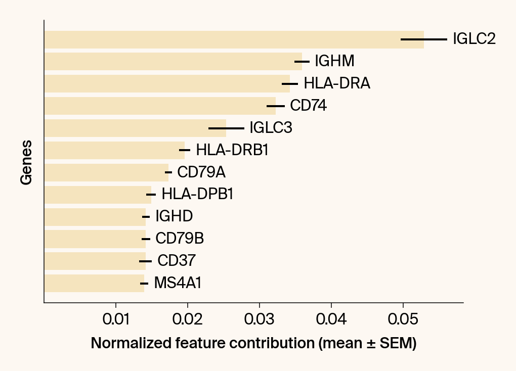
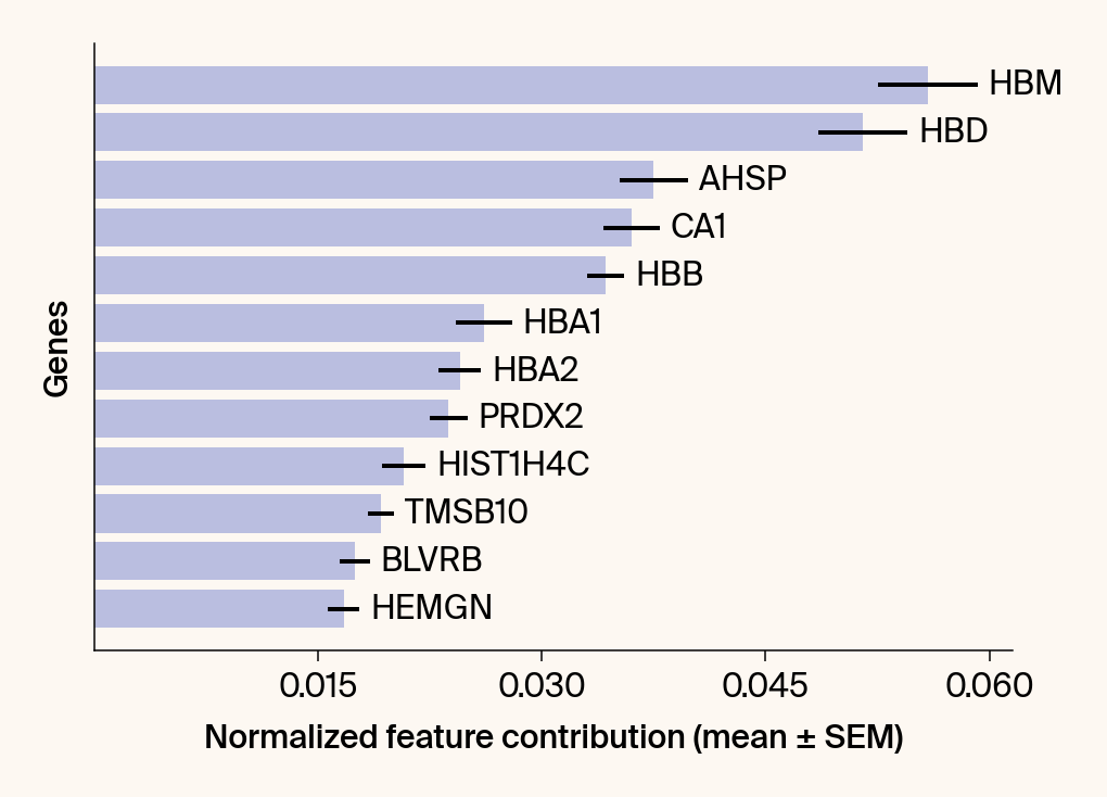
            # --- Plot 2: Bar chart ---
            
            # Create a new, separate figure
            fig2 = plt.figure()#figsize=[6, 6])
            
            # Use plt.barh
            bars = plt.barh(top_genes, top_means, xerr=top_sems, capsize=3, color=color_map.get(group, 'gray'))
            
            # Get current axis for bar_label, spines, and box_aspect
            current_ax = plt.gca()
            current_ax.bar_label(bars, labels=[f'{g}' for g in top_genes], padding=5)
            
            # Use plt.tick_params, xlabel, ylabel
            plt.tick_params(axis='y', left=False, labelleft=False)
            plt.xlabel("Normalized feature contribution (mean ± SEM)") 
            plt.ylabel("Genes")
            
            current_ax.spines[['right', 'top']].set_visible(False)
            if set_axes_equal:
                current_ax.set_box_aspect(1)
            current_ax.xaxis.set_major_locator(plt.MaxNLocator(nbins=6, prune='both'))
            fig2.tight_layout()
            plt.show()
            
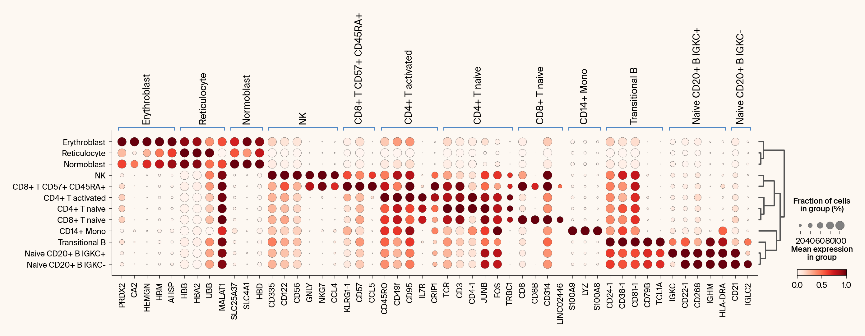
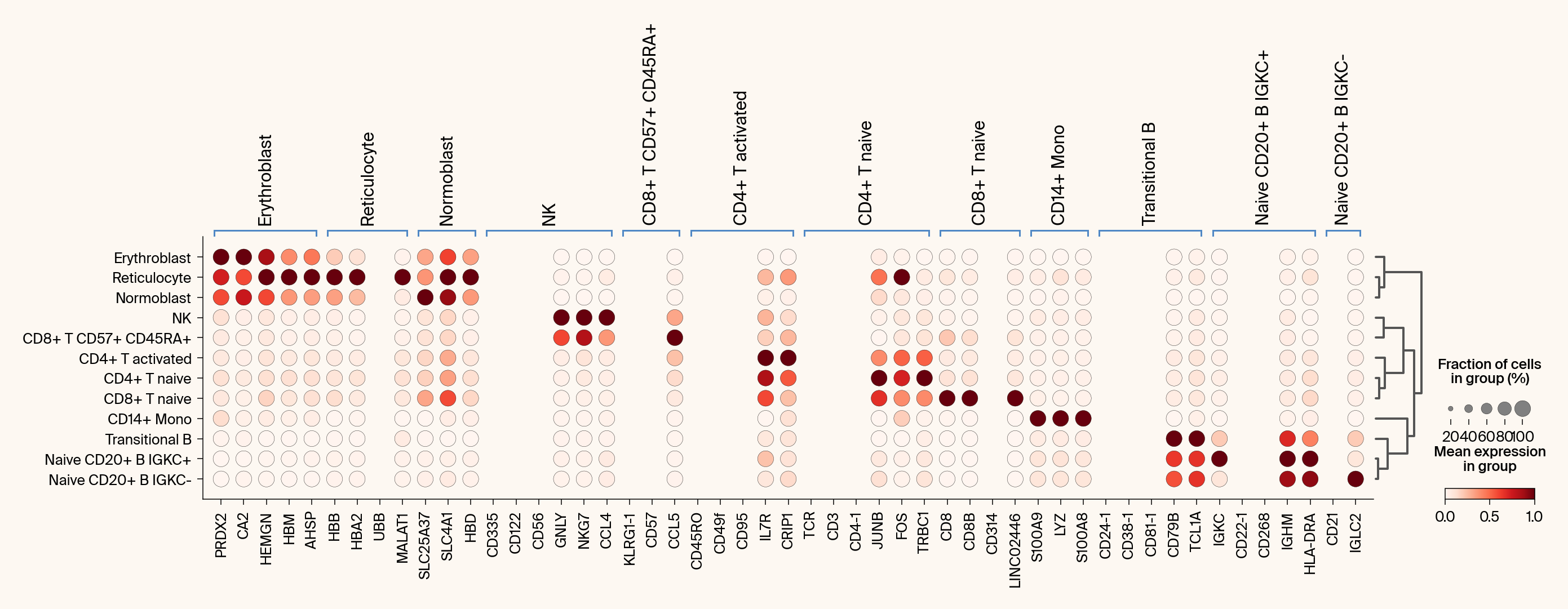
def compare_with_differential_expression(
    reducer: GlassBoxUMAP,
    adata: ad.AnnData,
    groupby: str = 'cell_type',
    n_top_genes: int = 2, 
    summary_stats_file: str = "analysis_summary_stats.csv",
    summary_plot_file: str = "analysis_summary_plot_data.npz" 
):
    """
    Compares Jacobian features with differential expression via dot plots.
    
    Args:
        reducer (GlassBoxUMAP): The fitted model object.
        adata (ad.AnnData): The processed AnnData object.
        groupby (str): The .obs column to use for grouping (e.g., 'cell_type').
    """
    import os
    from collections import defaultdict
    layer_to_use = None
    
    can_load_from_file = (
        summary_stats_file and os.path.exists(summary_stats_file) and
        summary_plot_file and os.path.exists(summary_plot_file)
    )
    
    if can_load_from_file:
        summary_df = pd.read_csv(summary_stats_file)
        
        jacobian_dict = {}
        for group in adata.obs[groupby].cat.categories:
            if group in summary_df[groupby].values:
                top_genes = summary_df[summary_df[groupby] == group].sort_values(
                    'mean_contribution', ascending=False
                )['gene'].values[:n_top_genes]
                jacobian_dict[group] = list(top_genes)
        
        with np.load(summary_plot_file, allow_pickle=True) as data:
            if 'jacobian_magnitude' not in data or 'gene_names' not in data:
                print("Warning: 'jacobian_magnitude' or 'gene_names' not found in summary file.")
            else:
                loaded_magnitude = data['jacobian_magnitude']
                loaded_genes = data['gene_names'] # Gene names from the NPZ file
                
                # Re-align loaded layer with current adata
                gene_to_npz_index = {gene: i for i, gene in enumerate(loaded_genes)}
                new_layer = np.zeros(adata.shape, dtype=loaded_magnitude.dtype)
                
                genes_found = 0
                for i, gene in enumerate(adata.var_names):
                    if gene in gene_to_npz_index:
                        new_layer[:, i] = loaded_magnitude[:, gene_to_npz_index[gene]]
                        genes_found += 1
                
                adata.layers['jacobian_magnitude'] = new_layer
                layer_to_use = 'jacobian_magnitude'
            
    else:
        if not reducer.feature_contributions_:
            raise RuntimeError("Must run compute_attributions() first to generate stats.")
        
        stats_df = reducer.get_feature_importance(adata, groupby, adata.var_names.values)
        
        jacobian_dict = {}
        for group in adata.obs[groupby].cat.categories:
            if group in stats_df[groupby].values:
                top_genes = stats_df[stats_df[groupby] == group].sort_values(
                    'mean_contribution', ascending=False
                )['gene'].values[:n_top_genes]
                jacobian_dict[group] = list(top_genes)
        
        jacobxall_first_run = reducer.feature_contributions_[0]
        adata.layers['jacobian_magnitude'] = np.linalg.norm(jacobxall_first_run, axis=1)
        layer_to_use = 'jacobian_magnitude'

    sc.tl.rank_genes_groups(adata, groupby=groupby, method="wilcoxon", n_genes=n_top_genes)

    de_dict = {
        name: list(adata.uns['rank_genes_groups']['names'][name])
        for name in adata.uns['rank_genes_groups']['names'].dtype.names
    }

    combined_genes = defaultdict(list)
    seen_genes = set()
    for d in (de_dict, jacobian_dict):
        for key, value in d.items():
            for gene in value:
                if gene not in seen_genes:
                    combined_genes[key].append(gene)
                    seen_genes.add(gene)
    
    with mpl.rc_context({"figure.facecolor": apc.parchment, "axes.facecolor": apc.parchment}):
        # Plot 1: Differential Expression
        ax1 = sc.pl.rank_genes_groups_dotplot(
            adata, var_names=combined_genes, groupby=groupby, 
            standard_scale="var", show=False
        )
        # plt.title("Differential expression (Combined DE + Jacobian Genes)")
        # plt.show()

        # Plot 2: Jacobian Feature Importance
        if layer_to_use:
            ax2 = sc.pl.rank_genes_groups_dotplot(
                adata, var_names=combined_genes, groupby=groupby, 
                layer=layer_to_use, standard_scale="var", show=False
            )
            # plt.title("Jacobian feature importance")
            # plt.show()
        else:
            print("Warning: Could not plot Jacobian dot plot. 'jacobian_magnitude' data was not found.")
        plt.show()

def set_fonts():
    """(Optional) Setup custom fonts."""
    font_files = fm.findSystemFonts('Suisse Int_l/')
    if len(font_files)>0:
        for font_file in font_files:
            fm.fontManager.addfont(font_file)

set_fonts()
setup_plotting_themes()

Since the PyTorch (v2.9.0) UMAP implementation is slightly different than the conventional UMAP (v0.5.9.post2), we generate the embeddings using both approach and show them below in Figure 1.

adata_final.obsm['X_parametric_umap_0'] = reducer.embeddings_[0]

plot_scanpy_umap(adata_final, groupby=GROUPBY_KEY)

plot_parametric_umap(reducer, adata_final, fit_index=0, groupby=GROUPBY_KEY)

(a) The conventional ScanPy (v1.11.4) UMAP embedding.

(b) The PyTorch (v2.9.0) network UMAP embedding.

Figure 1: The conventional ScanPy (v1.11.4) UMAP and the PyTorch (v2.9.0) network UMAP. It is also possible to directly fit the embedding learned by the conventional UMAP algorithm, but here we show a fit with the PyTorch (v2.9.0) method to demonstrate how they find similar embeddings.

Exact decomposition of features

The Jacobians are computed for each input over the independent fits. This takes a bit of time: about two minutes per fit on a GPU with 16 GB VRAM (on the order of the time spent fitting the model).

if TRAIN:
    adata_mean_zero = adata_final.to_df().values - adata_final.to_df().mean(axis=0).values
    
    reducer.compute_attributions(
        X_centered_gene_expression=adata_mean_zero,
        pca_components=adata_final.varm["PCs"]
    )
    print(SUMMARY_BASENAME)
    reducer.save_analysis_summary(adata_final, groupby=GROUPBY_KEY, basename=SUMMARY_BASENAME)

We can validate that the Jacobian reconstructs the embedding network output below in Figure 2.

validate_jacobian(
    reducer, 
    n_samples=200
)

(a) UMAP embedding position vs. the Jacobian reconstruction.

(b) Histogram of reconstruction error at float64. The max error is about 3e-14, approaching machine precision.

Figure 2: Jacobian reconstruction. To validate that the Jacobian reconstructs the UMAP encoder network output, we plot the embedding values against their Jacobian reconstructions and see that they fall on the identity line as well as the histogram of the reconstruction error.

PyTorch (v2.9.0) UMAP with Feature Labels

We can visualize the PyTorch (v2.9.0) embedding and add the top gene contributors to the embedding positions as information in the hovertip in Figure 3. The hovertip information provides feature contributions for each point in the dataset.

Embedding labeled by cell type

#plotly UMAP embedding with data tags

plot_interactive(
    reducer, 
    adata_final,
    groupby=GROUPBY_KEY,
    color_by='group', # or 'top_gene'
    fit_index=0,
    summary_file=summary_interactive_file if not TRAIN else None
)

Figure 3: The PyTorch (v2.9.0) UMAP embedding colored by cell type with top genes for each cell labeled in the hover tip.

Embedding labeled by top gene contributor

The embedding position can also be colored by the top gene contributor to the position for each cell as below in Figure 4. In some cases, a given cell type label may have different regions where different genes make the largest contribution. For example, the Normoblast class has two sub-regions, with the strongest contributors being HBD and HBB. Notably, the sub-region with HBD as the largest gene contributor also extends to the neighboring Erythroblast cluster.

#plotly UMAP embedding colored by top gene features
plot_interactive(
    reducer, 
    adata_final,
    groupby=GROUPBY_KEY,
    color_by='top_gene',
    fit_index=0,
    summary_file=summary_interactive_file if not TRAIN else None
)

Figure 4: The PyTorch (v2.9.0) UMAP embedding colored by top gene feature, showing that some cell types have regions with different top gene contributors, and some top gene contributors extend across type divisons. This plot only shows 84% of the points in the dataset, as the top features for the remaining points are more unique and would require a longer legend.

Top gene features by cell type

We can also generate plots for the average feature contribution for each class in Figure 5, similar to visualizations found in Chari and Pachter (2023). Note that the largest feature contributors do not always point in the direction of the centroid. This gives rise to a variation of contributions for that feature for individual cells across a cluster.

With 16 separate UMAP fits at different random initializations, we provide the standard error of the normalized mean contribution of each feature. The feature contributions are normalized by the mean embedding distance of the class for a given fit, since a class could be close to the origin for one fit, and far away from the origin in another fit.

group_to_plot = adata_final.obs[GROUPBY_KEY].value_counts().index[:12].tolist()
plot_feature_importance_by_group(
    reducer,
    adata_final,
    groupby=GROUPBY_KEY,
    groups_to_plot=group_to_plot,
    fit_index=0,
    summary_stats_file=summary_stats_file if not TRAIN else None,
    summary_plot_file=summary_plot_file if not TRAIN else None
)

(a) Reticulocyte, UMAP feature vectors for fit 0.

(b) Reticulocyte, UMAP feature length, mean over 16 fits.

(c) CD4+ T naive, UMAP feature vectors for fit 0.

(d) CD4+ T naive, UMAP feature lengths, mean over 16 fits.

(e) CD8+ T naive, UMAP feature vectors for fit 0.

(f) CD8+ T naive, UMAP feature lengths, mean over 16 fits.

(g) CD14+ mono, UMAP feature vectors for fit 0.

(h) CD14+ mono, UMAP feature lengths, mean over 16 fits.

(i) CD4+ T activated, UMAP feature vectors for fit 0.

(j) CD4+ T activated, UMAP feature lengths, mean over 16 fits.

(k) Naive CD20+ B IGKC+, UMAP feature vectors for fit 0.

(l) Naive CD20+ B IGKC+, UMAP feature lengths, mean over 16 fits.

(m) Naive CD20+ B IGKC-, UMAP feature vectors for fit 0.

(n) Naive CD20+ B IGKC-, UMAP feature lengths, mean over 16 fits.

(o) Erythroblast, UMAP feature vectors for fit 0.

(p) Erythroblast, UMAP feature lengths, mean over 16 fits.

(q) Normoblast, UMAP feature vectors for fit 0.

(r) Normoblast, UMAP feature lengths, mean over 16 fits.

(s) NK, UMAP feature vectors for fit 0.

(t) NK, UMAP feature lengths, mean over 16 fits.

(u) Transitional B, UMAP feature vectors for fit 0.

(v) Transitional B, UMAP feature lengths, mean over 16 fits.

(w) CD8+ T CD57+ CD45RA+, UMAP feature vectors for fit 0.

(x) CD8+ T CD57+ CD45RA+, UMAP feature lengths, mean over 16 fits.

Figure 5: The top gene features for each cell type. Note that the largest feature vectors do not always point to the centroid, often indicating a gradient of importance for that feature across the cluster. Error bars are generated by normalizing the feature importance vectors for each cell by the distance to the centroid of the class for that UMAP fit to account for changing cluster centroids across fits.

Dot plots

We can compare the features found by the Jacobian to differential expression with dot plots for each as in Figure 6.

We find that many features identified by differential expression between cell types are not preserved in the Jacobian representation. This highlights how the Jacobian method provides a complementary view of the feature space to features from differential expression.

import warnings
sc.settings.verbosity = 0
compare_with_differential_expression(
    reducer,
    adata_final,
    groupby=GROUPBY_KEY,
    n_top_genes=3,
    summary_stats_file=summary_stats_file if not TRAIN else None,
    summary_plot_file=summary_plot_file if not TRAIN else None
)

(a) The dot plot for the top differential expression features by cell type.

(b) The dot plot for the top Jacobian features by cell type.

Figure 6: Dot plots for gene expression analysis.

Conclusion

This work presents a novel approach to interpreting UMAP embeddings by utilizing glass-box deep networks. We have shown how to overcome the black-box nature of nonlinear dimensionality reduction for UMAP by implementing a locally linear (but globally nonlinear) embedding function. This enables the precise quantification of feature attributions for each data point in the UMAP embedding space, directly quantifying the contribution of individual genes to cell positions for gene expression data. This stands in contrast to conventional methods, such as differential expression, which provide only a proxy for what UMAP has learned.

References

Arcadia-pycolor. (2025)

Chari T, Pachter L. (2023). The specious art of single-cell genomics. https://doi.org/10.1371/journal.pcbi.1011288

Elhage N, Nanda N, Olsson C, Henighan T, Joseph N, Mann B, Askell A, Bai Y, Chen A, Conerly T, DasSarma N, Drain D, Ganguli D, Hatfield-Dodds Z, Hernandez D, Jones A, Kernion J, Lovitt L, Ndousse K, Amodei D, Brown T, Clark J, Kaplan J, McCandlish S, Olah C. (2021). A mathematical framework for transformer circuits

Golden JR. (2025). Equivalent linear mappings of large language models

Luecken MD, Burkhardt DB, Cannoodt R, Lance C, Agrawal A, Aliee H, Chen AT, Deconinck L, Detweiler AM, Granados AA, others. (2021). A sandbox for prediction and integration of DNA, RNA, and proteins in single cells

Lundberg SM, Lee S-I. (2017). A unified approach to interpreting model predictions. https://doi.org/10.48550/arXiv.1705.07874

McInnes L, Healy J, Melville J. (2018). Umap: Uniform manifold approximation and projection for dimension reduction. https://doi.org/10.48550/arXiv.1802.03426

Mohan S, Kadkhodaie Z, Simoncelli EP, Fernandez-Granda C. (2019). Robust and interpretable blind image denoising via bias-free convolutional neural networks. https://doi.org/10.48550/arXiv.1906.05478

Ng S, Masarone S, Watson D, Barnes MR. (2023). The benefits and pitfalls of machine learning for biomarker discovery. https://doi.org/10.1007/s00441-023-03816-z

Pascarelli E. (2023). umap-pytorch: Pytorch port for parametric umap

Ribeiro MT, Singh S, Guestrin C. (2016). Why should i trust you? Explaining the predictions of any classifier. https://doi.org/10.48550/arXiv.1602.04938

Sainburg T, McInnes L, Gentner TQ. (2021). Parametric UMAP embeddings for representation and semisupervised learning. https://doi.org/10.1162/neco_a_01434

Selvaraju RR, Cogswell M, Das A, Vedantam R, Parikh D, Batra D. (2017). Grad-cam: Visual explanations from deep networks via gradient-based localization. https://doi.org/10.48550/arXiv.1610.02391

Wang S, Mohamed A-R, Caruana R, Bilmes J, Plilipose M, Richardson M, Geras K, Urban G, Aslan O. (2016). Analysis of deep neural networks with the extended data jacobian matrix

Wolf FA, Angerer P, Theis FJ. (2018). SCANPY: Large-scale single-cell gene expression data analysis. https://doi.org/10.1186/s13059-017-1382-0

York R, Mets DG. (2025). G–P Atlas: A neural network framework for mapping genotypes to many phenotypes. https://doi.org/10.57844/arcadia-d316-721f